Contents

function wave

% WAVE solves the wave equation
%                   u_{tt} = c^2 u_{xx}
% using central spatial differences and the method of lines.
% Write the equation as first-order system for U = [u, v]
%                   u_t = v,    v_t = c^2 u_{xx}
% and use periodic boundary conditions.
%==========================================================================

clear all;
close all;

Set time parameters

c = 1.;                                                                     % wave speed
t0 = 0.;                                                                    % initial time
tf = 4.;                                                                    % final time
lt = 200;                                                                   % number of times to output solution
dtplot = (tf-t0)/lt;
tspan = t0:dtplot:tf;
lt = length(tspan);

Set space parameters

x0 = -8;                                                                    % left endpoint
x1 = 8;                                                                     % right endpoint
ord = 10;                                                                   % n = 2^ord spatial grid points
pltord = 8;                                                                 % use 2^pltord points for surface plots
xlength = x1-x0;
nord = 2^ord;
dx = xlength/nord;
x = x0+dx*(0:(nord-1));
lx = length(x);

Set initial condition u0 = u(x,0), u_t0 = u_t(x,0)

u0 = uzero(x,lx);
u_t0 = utzero(x,lx);
U0 = [u0,u_t0].';
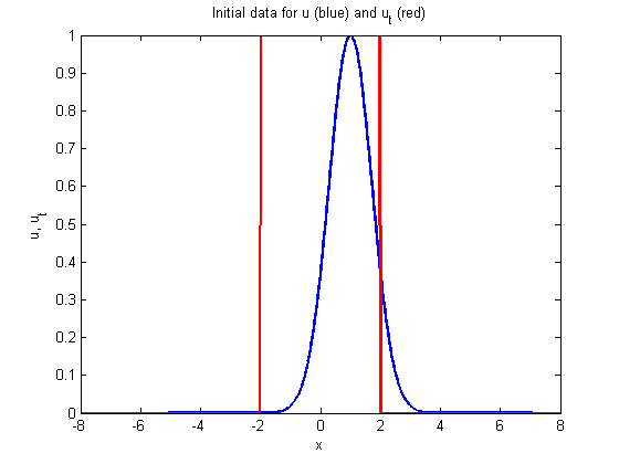
figure(1)
plot(x,u0,'b-',x,u_t0,'r-')
xlabel('x'); ylabel('u, u_t');
title('Initial data for u (blue) and u_t (red)')

Solve the equation

options = odeset('AbsTol', 1.0e-6, 'RelTol', 1.0e-3);
[t, U] = ode45(@fw,tspan,U0,options,c,lx,dx);

Plot the solution

nwater=1; ncontour=1;  nenergy=1; nmovie=0; ngraph=1;                       % flags for different plots
                                                                            % set equal to 1 to plot
u = U(:,1:lx);
u_t = U(:,lx+1:2*lx);
umax = max(max(u));
umin = min(min(u));
pltord = min(pltord,ord);
dxplot = 2^(ord-pltord);
nxplot = 1:dxplot:lx;
xplot = x(nxplot);
uplot = u(:,nxplot);

Surface plot

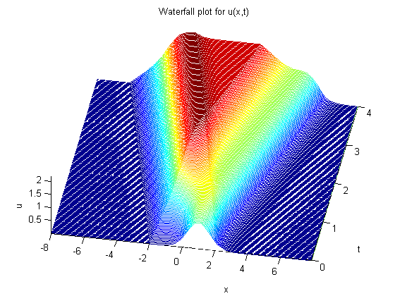
if (nwater==1)
    figure(2);                                                              % waterfall plot
    waterfall(xplot,t,uplot)
    view(10,70)
    axis tight
    xlabel('x'), ylabel('t'), zlabel('u')
    title('Waterfall plot for u(x,t)')
    grid off
end

if (ncontour==1)
    figure(3);  clf;                                                        % contour plot
    contour(xplot,t,uplot,40)
    xlabel('x'), ylabel('t'), title('Contour plot for u(x,t)')
end

Energy plot

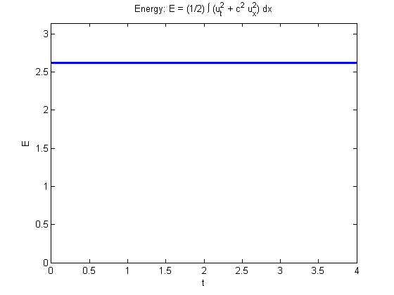
if (nenergy==1)
    figure(4);   clf;                                                       % energy (1/2) \int (u_t^2 + c^2 u_x^2) dx
    e=zeros(1,lt);
    for j=1:lt
        uj = u(j,:);
        ujp = circshift(uj.',1).';
        ujx = (ujp - uj)/dx;
        ujt = u_t(j,:);
        e(j) = 0.5*dx*(sum(ujt.^2) + c^2*sum(ujx.^2));
    end
    plot(t,e);
    emax=max(0,1.2*max(e)); emin = min(0,1.2*min(e));
    axis ([t0 tf emin emax]);
    title('Energy: E = (1/2) \int (u_t^2 + c^2 u_x^2) dx');
    xlabel('t'); ylabel('E');
end

Movie plots

if (nmovie==1)                                                              % generates movie
        textx = x1 - (x1-x0)/4;
        textu = umax - (umax-umin)/10;
        figure(5);
        mvplotu=moviein(lt);
        hold off;
        for jj = 1:lt
            umplot = u(jj,:);
            plot(x,umplot);
            axis([x0 x1 umin umax]);
            xlabel('x'); ylabel('u');
            text(textx,textu,strcat('time = ',num2str(t(jj))));
            mvplotu(jj) = getframe(gcf);
        end
        movie2avi(mvplotu,'u.avi',...
            'fps',25,'quality',100,'compression','None');
end

Solution at different times

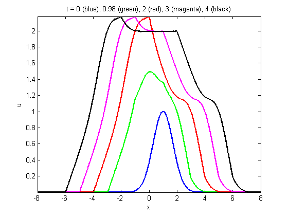
if (ngraph==1)
        j1 = round(lt/4); j2 = round(lt/2); j3 = round(3*lt/4);
        t0 =t(1); t1 = t(j1); t2 = t(j2); t3 = t(j3); t4 = t(lt);
        figure(6);
        plot(x,u(1,:),'b',x,u(j1,:),'g',x,u(j2,:),'r',...
             x,u(j3,:),'m',x,u(lt,:),'k');
        xlabel('x'); ylabel('u');
        axis([x0 x1 umin umax]);
        title(['t = ',num2str(t0),' (blue), ',...
               num2str(t1),' (green), '...
               num2str(t2),' (red), '...
               num2str(t3),' (magenta), '...
               num2str(t4),' (black)'])
end

end

Right-hand side of ODE for wave equation

function U_t = fw(~,U,c,lx,dx)
% FW gives right hand side of ODE for method of lines
u = U(1:lx);
u_t = U(lx+1:2*lx);
up = circshift(u,1);
un = circshift(u,-1);
du = u_t;
du_t = c^2*(up - 2*u + un)/dx^2;
U_t = [du; du_t];
end

Initial data for u

function u0 = uzero(x,lx)
% UZERO gives initial data for u
u0 = 0.*x;
for ii=1:lx
    if (x(ii)>-3) && (x(ii) < -2)
        u0(ii) = x(ii)+3;
    elseif (x(ii)>=-2) && (x(ii) < -1)
        u0(ii) = -1-x(ii);
    elseif (x(ii)>2) && (x(ii) < 3)
        u0(ii) = x(ii)-2;
    elseif (x(ii)>=3) && (x(ii) < 4)
        u0(ii) = 4-x(ii);
    else
        u0(ii) =0.;
    end
end
u0 = exp(-(x-1).^2);
%u0 = cos(pi*x/16);
%u0=0.*x;
end

Initial data for u_t

function u_t0 = utzero(x,lx)
% UTZERO gives initial data for u_t
u_t0 = 0.*x;
for ii=1:lx
    if (x(ii)>-2) && (x(ii) < 2)
        u_t0(ii) = 1.;
    else
        u_t0(ii) = 0.;
    end
end
%u_t0=0.*x;
end

Published with MATLAB® R2013a