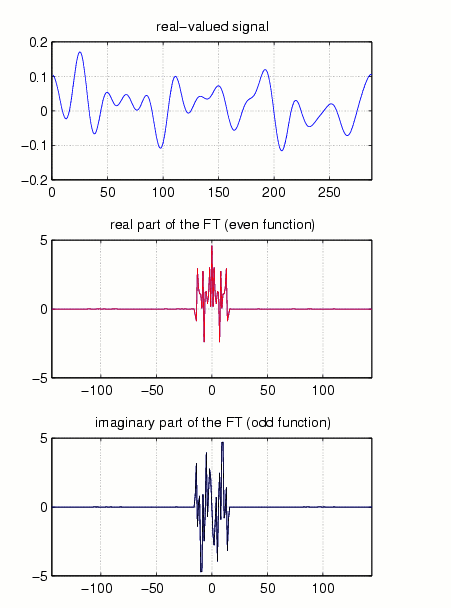
Let us first describe the situation for the one-dimensional case of vectors of finite length. Such a vector (real- or complex-valued) x[n] has spectrum in some set Omega (of its frequency domain) if all of the Fourier coefficients of x[n] which correspond to parts of the frequency domain outside Omega are zero. Typically, Omega will be some interval around the "origin" of the frequency domain.
Fig.1
(To distinguish the signal x[n] from its samples, see below,
we draw it as a continuous signal. For more details about the Fast Fourier
Transform and Labelling in MATLAB consult "The FFT-Guide".)
Fig.2
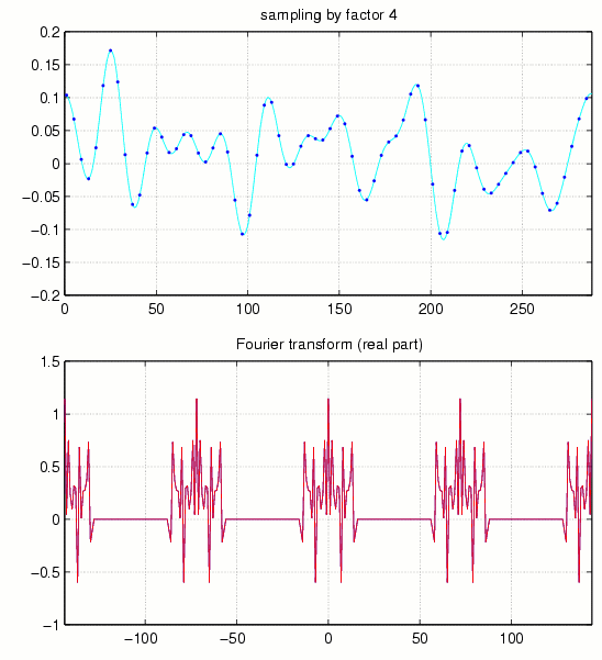
This indicates that complete reconstruction of the signal x[n] from such a periodized spectrum should be easily possible as long as the shifted copies of the spectrum y[k] do not overlap. The periodization constant being exactly N/a for a given sampling rate a, it turns out that the sampling rate should satisfy the so-called Nyquist criterion a<=N/M. For fixed Omega, any band-limited signal with spectrum in Omega can be completely reconstructed from regular samples, as long as the shifted versions of Omega (in the cyclic sense, by multiples of N/a) do not overlap with Omega. Indeed, in this case one simply has to multiply y_s[k] by some sequence h, with h(omega) == 1 for omega in Omega, and zero on all those shifted copies of Omega. Explicitly, if Omega is an interval of length M=30, then any divisor a of N will do which satisfies aM <= N, see also Fig.3:
Fig.3
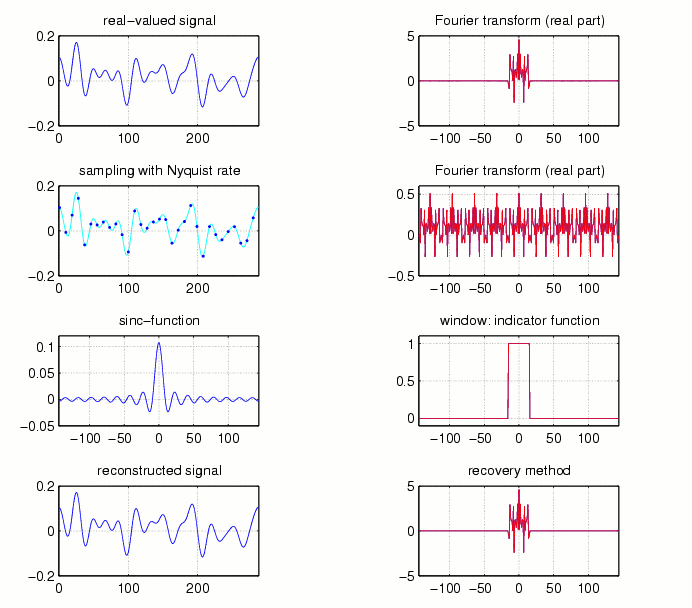
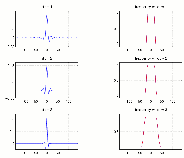
Since multiplication on the frequency side corresponds to convolution on the time-side, it is of interest also to have a look at the ''window'' g whose Fourier transform equals a given sequence, h=fft(g), for different choices of h. Fig.4 gives three examples of such windows, for the case N = 288 and M=30.
Fig.4
For the case of critical sampling (aM = N), cf. Fig.2,
the shifted copies of Omega are sitting side by side and there is
no other choice for h than the indicator function of Omega.
In this case g is just (a discrete variant) of the well-known SINC
function, which, however, is known to have fairly poor decay properties.
In contrast, for the case of ''oversampling'' (where one has more samples
than absolutely necessary), i.e. a is smaller than N/M, N/a
will be large compared to Omega. This gives some freedom in
the choice of h (instead of an indicator function one can e.g. choose
a trapezoid like function with decent decay at the ends). The corresponding
window g of a smooth function h will be better concentrated
near the origin.
Since convolution of the sampled signal with the window g can
be reinterpreted as forming a series of shifted copies of g, with
the given sampling coordinates being the coefficients of the series expansion
(linear combination), the better decay of g will result in better
locality properties of the reconstruction algorithm. In other words,
it is not necessary to have all the samples available in order to reconstruct
a part of a signal. The use of well localized ''atoms'' g
implies that the following (very natural) principle applies, indicating
that the truncation error can be reasonably kept within limits: Given some
interval of interest it is only necessary to use the samples in some neighborhood
of the given interval in order to achieve a small reconstruction error
there, see Fig.5:
Fig.5
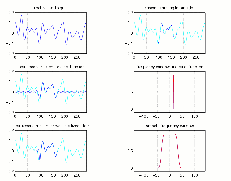
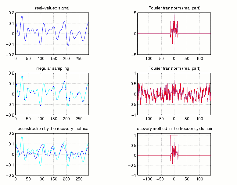
Fig.6
Most of the irregular sampling algorithms are iterative in nature.
Starting from some initial guess, typically based on the given sampling
values, further approximations are obtained step by step, using the available
(assumed) knowledge about the size and location of Omega (in some
cases an educated guess concerning Omega has to be made).
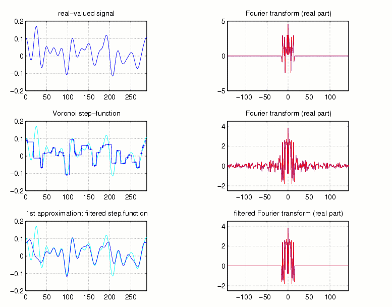
As a first example, let us explain the so-called Voronoi-method.
Here we start with nearest neighborhood interpolation. In other words,
given the sampling values at known positions we form a step function which
is constant from midpoint to midpoint of the given sampling sequence.
In the case where the number of missing points between subsequent sampling
positions is odd, the midpoint itself is assigned the arithmetic mean of
the two adjacent sampling points. Because of the assumed smoothness
of the signal, this step function will not be too far away from the original
signal, in the mean-squared sense. Having used the sampling values,
the information concerning Omega can be used next. The step
function (which appearently contains many high frequencies outside of Omega)
is filtered, i.e. only those Fourier coefficients which belong to Omega
are preservered, the rest is discarded. This operation corresponds
to a simple projection operator.
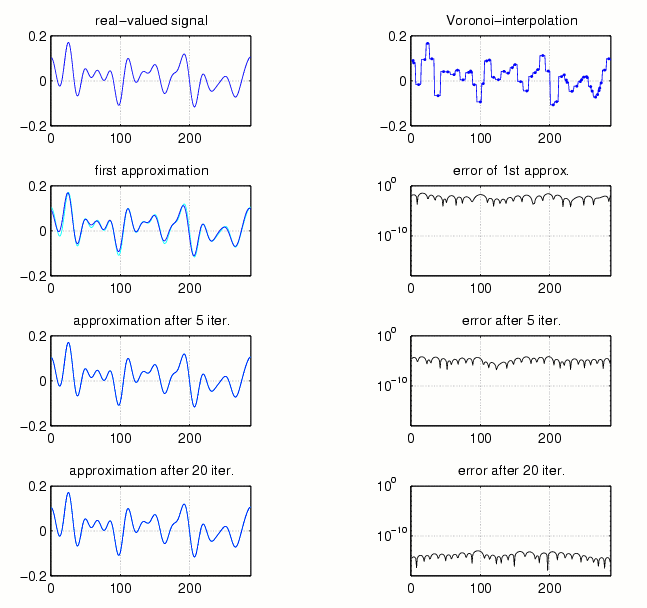
Fig.7 shows this step-function, the original sampling points plotted
as black points, and its Fourier transform in the first line. Below,
the filtered version is displayed. It is the first step of the iterative
Voronoi approach (or Allebach-algorithm).
Fig.7
Clearly the filtering process destroys the pointwise interpolation property
of the Voronoi step-function, but theoretical considerations show that
(given Omega and the sampling rate in terms of the maximal gap)
one can give the following guarantee: If the maximal gap is smaller
than the Nyquist rate (N/M), then the following iterative scheme
will converge to the original signal
x[n] at a geometric rate (which
will be the better the smaller the actual maximal gap is compared to the
Nyquist rate).
Indeed, it can be shown that there is some factor q < 1,
such that the Omega-filtered version x_1[n] of the nearest
neighborhood interpolation satisfies ||x-x_1|| < q
||x||. We therefore look at the difference signal x[n]-x_1[n].
According to the construction, x_1[n] has its spectrum within the
same set Omega, and for obvious reasons we know its coordinates
at the given sampling positions. Therefore, the estimate indicated
above can be applied and we can again recover a certain portion of the
remaining signal by repeating the first step, now starting with the sampled
coordinates of x[n]-x_1[n]. Technically speaking we
recover 100(1-q) percent of the missing energy of the difference
signal x[n]-x_1[n] at the second step. Continuing to
use the difference between the given sampling values of x[n] and
those of the n-th approximation we generate additive corrections which
lead stepwise to improved approximations.
Fig.8 shows the approximations of the Allebach-algorithm and their errors after 1, 5, and 20 iterations.
Fig.8
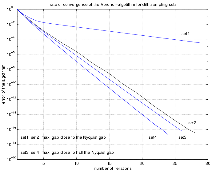
To give an idea of the rate of convergence depending on the maximal gap of the sampling set, Fig.9 compares four sampling sets by using the Voronoi-Allebach algorithm (set2 corresponds to the sampling set used in Fig.8).
Fig.9
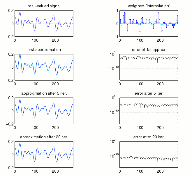
The Voronoi-approach is just one method to get a bandlimited approximation of the original signal from its sampling points. As one can guess, there exist some more. Indeed, if we use either a trivial interpolation (where all the unknown points are set equal to zero) or the so-called adaptive-weights-approximation (where every sample point is multiplied with a weight-factor depending on its distance to its neighbor sampling points), and if we proceed as in the Allebach-algorithm, then we get to other reconstruction methods known as the Marvasti-algorithm and the adaptive-weights-algorithm, respectively. To prove their convergence one can apply the same arguments as for the Voronoi-Allebach-algorithm.
Fig.10 and Fig.11 show the approximations and the corresponding errors of the two algorithms after 1, 5, and 20 iterations.
Fig.10: Marvasti-algorithm
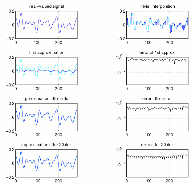
Fig.11: adaptive-weights-algorithm
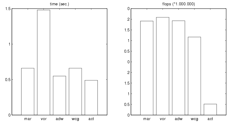
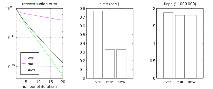
In order to visualize the difference between those algorithms, Fig.12 compares rates of convergence in terms of the reconstruction error, time, and number of floating point operations used for 20 iterations of the Voronoi-Allebach-algorithm (vor), the Marvasti-algorithm (mar), and the adaptive-weights-algorithm (adw) for the sampling sequence used in Fig.8, Fig.10, and Fig.11 .
Fig.12
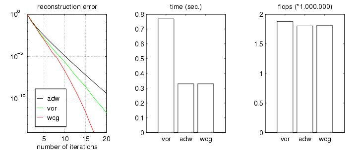
The adaptive-weights-method can be improved by using the conjugate gradient algorithm (cg), a very efficient method to solve iteratively a positive definite, symmetric, linear system. In fact, the first step of the adw-algorithm consisting of discarding high frequencies of the "weighted interpolation" of the signal x[n] in order to get the first approximatio x_1[n], can be replaced by the matrix- multiplication Sx=x_1, where S is of the form S=CC'. Let P be the number of irregular samples, then C is an (N,P)-matrix whose columns are the shifted (by the sampling points) versions of an appropriate atom on the time-side, C' denotes the transpose of C. It can be shown that S is positive definite and symmetric (Frame-theory). Applying the cg-method to Sx=x_1 in order to approximate the signal x[n] leads to the adaptive-weights-conjugate-gradient-algorithm (wcg). Note that S is completely determined by the known sampling information.
Fig.13 compares the wcg-algorithm with the Voronoi-method and the adaptive-weights-algorithm.
Fig.13:
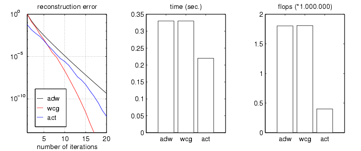
In the discrete case a band-limited signal can be written as a trigonometric polynomial. Using the Dirichlet kernel as atom on the time-side and introducing trigonometric polynomials, the linear system Sx=x_1 can be transformed into a system of a positive definite Toeplitz matrix, a matrix whose entries are constant along each diagonal. For the solution of such Toeplitz systems the cg-algorithm is an even more powerful acceleration method. The combination of adaptive weights, conjugate gradient, and Toeplitz systems forms the adaptive-conjugate-Toeplitz-algorithm (act), which is a very efficient iterative algorithm to reconstruct a band-limited signal from irregular sampling values.
The comparison between the adw-method, the wcg-method, and the act-algorithm is shown in Fig.14 .
Fig.14:
As a last example we compare all the algorithms mentioned above by taking a sampling sequence whose maximal gap is three times larger than the Nyquist gap, such that no theoretical guarantee for convergence can be given. In case of convergence the behavior of the error in terms of iterations can be considered as a mesure of stability.
Fig.15:
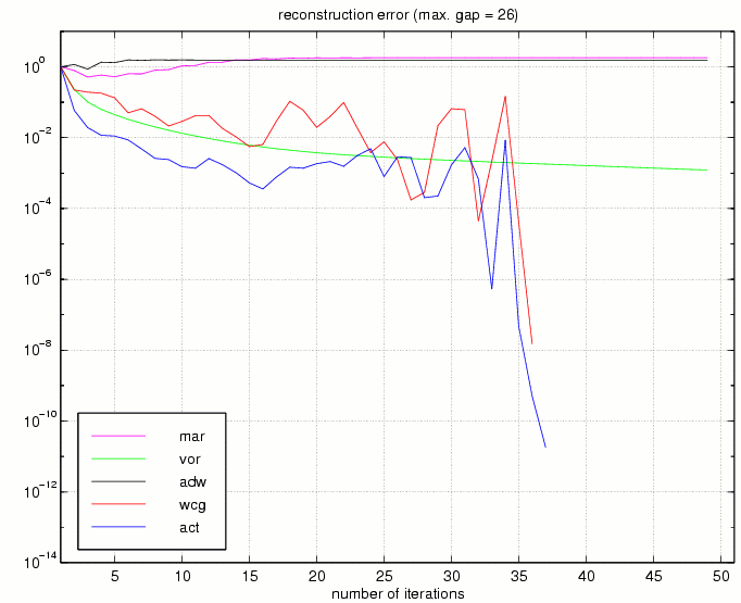
Fig.16: