sage.geometry.polyhedron
Matthias Köppe (UC Davis)
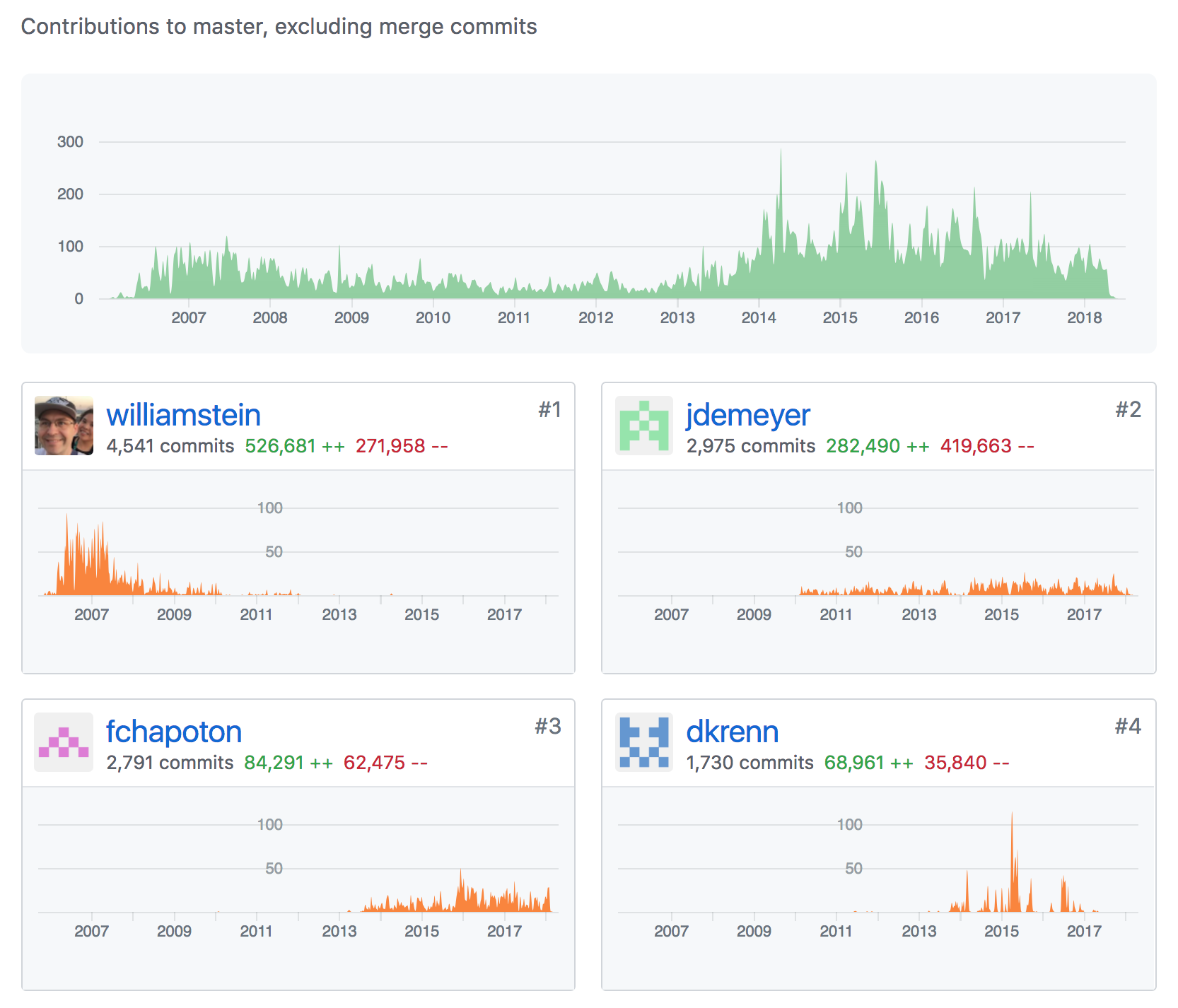
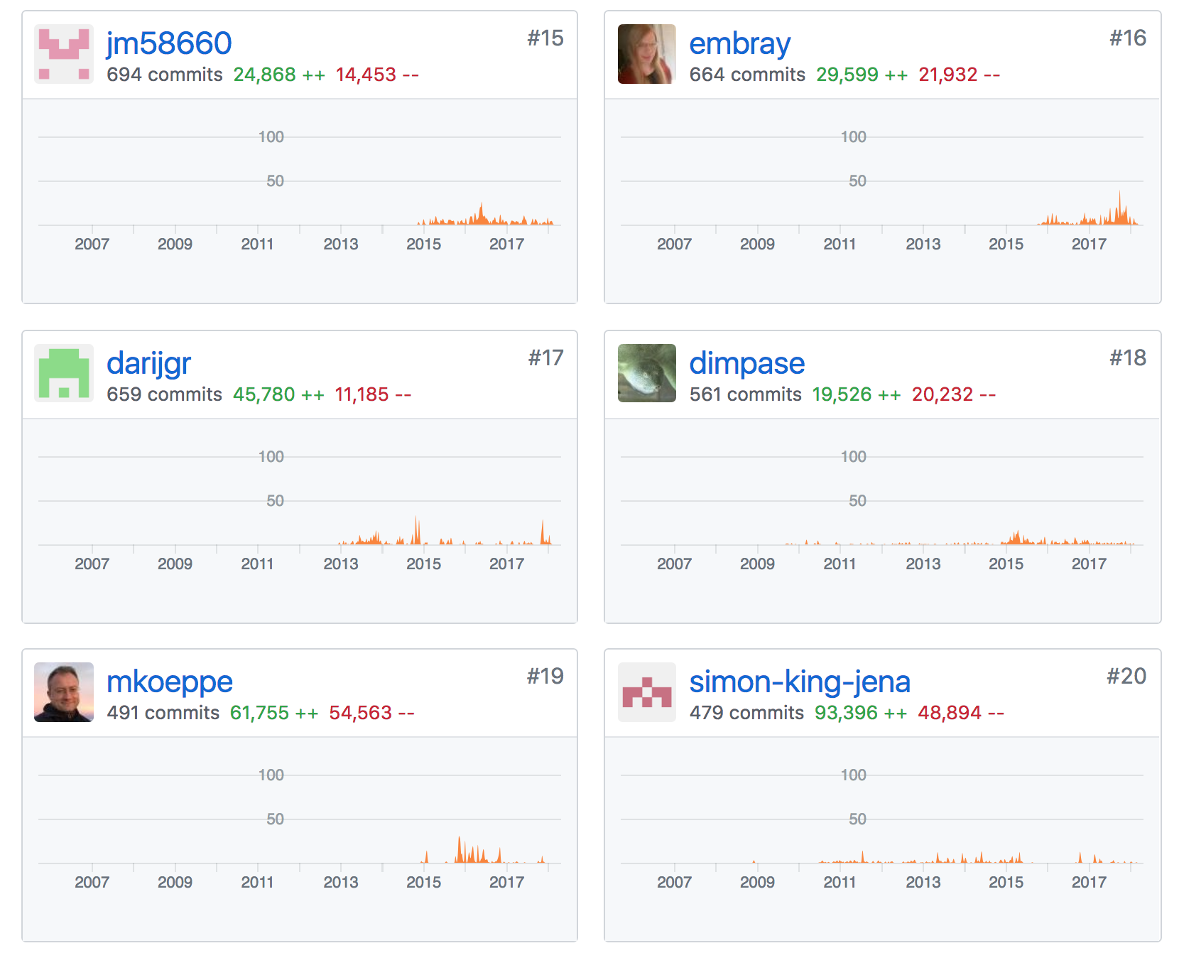
Software: based on 15 years of SageMath development (Stein et al., 2004-).
Talk: based in part on SageMath tutorials
My contributions:
Long-term maintenance of software packages 4ti2 (Hemmecke et al. 2001-), LattE integrale (De Loera et al. 2002-)
Some contributions to SageMath since 2015 (polyhedra, optimization, build system)
scrolling down …
Quick introduction to SageMath
What is SageMath?
- “Python with mathematical batteries included”
- Python extended through its metaobject protocol by an object system driven by “categories” and “axioms”, similar to Axiom and Magma
- With less emphasis, also has general untyped symbolics, provided by SymPy, Maxima, etc.
- Free software (GNU General Public License)
Two faces of SageMath:
sage-the-Python-library:
find src/sage -name "[a-z]*.py" -o -name "*.pyx" -o -name "*.pyd" | xargs wc -l

    263 src/sage/algebras/affine_nil_temperley_lieb.py
     38 src/sage/algebras/algebra.py
     69 src/sage/algebras/all.py
    343 src/sage/algebras/associated_graded.py
    110 src/sage/algebras/catalog.py
    326 src/sage/algebras/cellular_basis.py
   2840 src/sage/algebras/clifford_algebra.py
   2418 src/sage/algebras/cluster_algebra.py
   ...
    433 src/sage/geometry/polyhedron/backend_cdd.py
    268 src/sage/geometry/polyhedron/backend_field.py
    833 src/sage/geometry/polyhedron/backend_normaliz.py
    461 src/sage/geometry/polyhedron/backend_polymake.py
    266 src/sage/geometry/polyhedron/backend_ppl.py
   6970 src/sage/geometry/polyhedron/base.py
   ...
    340 src/sage/typeset/symbols.py
    161 src/sage/typeset/unicode_art.py
      5 src/sage/version.py
2163533 total
sage-the-software-distribution:
ls -1 build/pkgs/ && ls build/pkgs | wc -l

4ti2
alabaster
appnope
arb
atlas
...
polymake
polytopes_db
ppl
...
zlib
zn_poly
zope_interface
     286
Self-contained, just needs a compiler and build essentials to bootstrap (XCode command-line tools on macOS).
Installation:
Ignore binary distributions and source tarballs
Follow the instructions :ref: (Git the hard way) to checkout and build from source… or the following simplified instructions:
Check out most recent release:
[user@localhost ~]$ git clone --origin trac --single-branch \
  git://trac.sagemath.org/sage.git
Or, check out development version (current beta):
[user@localhost ~]$ git clone --origin trac --single-branch \
  --branch develop git://trac.sagemath.org/sage.git
Build:
[user@localhost ~]$ cd sage
[user@localhost sage]$ MAKE='make -j8' make
By tomorrow it will be finished
Start it:
[user@localhost sage]$ ./sage
Then interact using the IPython REPL.
Other options:
- Ubuntu has sage packages
- Other Linux distros: https://repology.org/metapackage/sagemath/versions
- cocalc.com
- Docker images: sagemath, cocalc
- conda
How to contribute to SageMath
- Change tickets at http://trac.sagemath.org with technical discussion
- Log in to http://trac.sagemath.org with your GitHub account
- Create branch, make changes, build, run test suite, commit, create or update Trac ticket, push branch to ticket, set to “needs review”, wait for / find peer reviewer …
Introduction to polyhedral computation facilities in SageMath
(Adapted from the tutorial “A Longer Introduction to Polyhedral Computations in Sage” in the SageMath documentation, written by Jean-Philippe Labbé <labbe@math.fu-berlin.de> during the SageDays 84 in Olot (Spain).)
Basic definitions and constructions
A real \((k\times d)\)-matrix \(A\) and a real vector \(b\) in \(\mathbb{R}^d\) define a (convex) polyhedron \(P\) as the set of solutions of the system of linear inequalities:
Each row of \(A\) defines a closed half-space of \(\mathbb{R}^d\). Hence a polyhedron is the intersection of finitely many closed half-spaces in \(\mathbb{R}^d\). The matrix \(A\) may contain equal rows, which may lead to a set of equalities satisfied by the polyhedron. If there are no redundant rows in the above definition, this definition is referred to as the \(\mathbf{H}\) -representation of a polyhedron.
A maximal affine subspace \(L\) contained in a polyhedron is a lineality space of \(P\). Fixing a point \(o\) of the lineality space \(L\) to act as the origin, one can write every point \(p\) inside a polyhedron as a combination
where \(\sum_{i=1}^n\lambda_i=1\), \(\lambda_i\geq0\), \(\mu_i\geq0\), and \(r_i\neq0\) for all \(0\leq i\leq m\) and the set of \(r_i\) ‘s are positively independent (the origin is not in their positive span). For a given point \(p\) there may be many equivalent ways to write the above using different sets \(\{v_i\}_{i=1}^{n}\) and \(\{r_i\}_{i=1}^{m}\). Hence we require the sets to be inclusion minimal sets such that we can get the above property equality for any point \(p\in P\).
The vectors \(v_i\) are called the vertices of \(P\) and the vectors \(r_i\) are called the rays of \(P\). This way to represent a polyhedron is referred to as the \(\mathbf{V}\) -representation of a polyhedron. The first sum represents the convex hull of the vertices \(v_i\) ‘s and the second sum represents a pointed polyhedral cone generated by finitely many rays.
When the lineality space and the rays are reduced to a point (i.e. no rays and no lines) the object is often referred to as a polytope.
Note
As mentioned in the documentation of the constructor when typing Polyhedron?:
You may either define it with vertex/ray/line or inequalities/equations data, but not both. Redundant data will automatically be removed (unless “minimize=False”), and the complementary representation will be computed.
\(V\)-representation
First, let’s define a polyhedron object as the convex hull of a set of points and some rays.
sage: P1 = Polyhedron(vertices = [[1, 0], [0, 1]], rays = [[1, 1]])
sage: P1
A 2-dimensional polyhedron in ZZ^2 defined as the convex hull of 2 vertices and 1 ray
The string representation already gives a lot of information:
- the dimension of the polyhedron (the smallest affine space containing it)
- the dimension of the space in which it is defined
- the base ring (\(\mathbb{Z}^2\)) over which the polyhedron lives (this specifies the parent class, see sage.geometry.polyhedron.parent)
- the number of vertices
- the number of rays
We can also add a lineality space.
sage: P2 = Polyhedron(vertices = [[1/2, 0, 0], [0, 1/2, 0]],
....:                 rays = [[1, 1, 0]],
....:                 lines = [[0, 0, 1]])
sage: P2
A 3-dimensional polyhedron in QQ^3 defined as the convex hull of 2 vertices, 1 ray, 1 line
Notice that the base ring changes because of the value \(\frac{1}{2}\). Indeed, Sage finds an appropriate ring to define the object.
sage: P1.parent()
Polyhedra in ZZ^2
sage: P2.parent()
Polyhedra in QQ^3
\(H\)-representation
If a polyhedron object was constructed via a \(V\)-representation, Sage can provide the \(H\)-representation of the object.
sage: for h in P1.Hrepresentation():
....:     print(h)
An inequality (1, 1) x - 1 >= 0
An inequality (1, -1) x + 1 >= 0
An inequality (-1, 1) x + 1 >= 0
Each line gives a row of the matrix \(A\) and an entry of the vector \(b\).
The variable \(x\) is a vector in the ambient space where P1 is
defined. The \(H\)-representation may contain equations:
sage: P3.Hrepresentation()
(An inequality (-2.0, 0.0) x + 1.0 >= 0,
 An inequality (1.0, 0.0) x + 0.0 >= 0,
 An equation (1.0, 1.0) x - 0.5 == 0)
The construction of a polyhedron object via its \(H\)-representation,
requires a precise format. Each inequality \((a_{i1}, \dots, a_{id})\cdot
x + b_i \geq 0\) must be written as [b_i,a_i1, ..., a_id].
sage: P3_H = Polyhedron(ieqs = [[1.0, -2, 0], [0, 1, 0]], eqns = [[-0.5, 1, 1]])
sage: P3 == P3_H
True
sage: P3_H.Vrepresentation()
(A vertex at (0.0, 0.5), A vertex at (0.5, 0.0))
It is worth using the parameter eqns to shorten the construction of the
object. In the following example, the first four rows are the negative of the
second group of four rows.
sage: H = [[0, 0, 0, 0, 0, 0, 0, 0, 1],
....:  [0, 0, 0, 0, 0, 0, 1, 0, 0],
....:  [-2, 1, 1, 1, 1, 1, 0, 0, 0],
....:  [0, 0, 0, 0, 0, 0, 0, 1, 0],
....:  [0, 0, 0, 0, 0, 0, 0, 0, -1],
....:  [0, 0, 0, 0, 0, 0, -1, 0, 0],
....:  [2, -1, -1, -1, -1, -1, 0, 0, 0],
....:  [0, 0, 0, 0, 0, 0, 0, -1, 0],
....:  [2, -1, -1, -1, -1, 0, 0, 0, 0],
....:  [0, 0, 0, 0, 1, 0, 0, 0, 0],
....:  [0, 0, 0, 1, 0, 0, 0, 0, 0],
....:  [0, 0, 1, 0, 0, 0, 0, 0, 0],
....:  [-1, 1, 1, 1, 1, 0, 0, 0, 0],
....:  [1, 0, 0, -1, 0, 0, 0, 0, 0],
....:  [0, 1, 0, 0, 0, 0, 0, 0, 0],
....:  [1, 0, 0, 0, -1, 0, 0, 0, 0],
....:  [1, 0, -1, 0, 0, 0, 0, 0, 0],
....:  [1, -1, 0, 0, 0, 0, 0, 0, 0]]
sage: timeit('Polyhedron(ieqs = H)')  # random
125 loops, best of 3: 5.99 ms per loop
sage: timeit('Polyhedron(ieqs = H[8:], eqns = H[:4])')  # random
125 loops, best of 3: 4.78 ms per loop
sage: Polyhedron(ieqs = H) == Polyhedron(ieqs = H[8:], eqns = H[:4])
True
Of course, this is a toy example, but it is generally worth to preprocess the data before defining the polyhedron if possible.
Representation objects
Many objects are related to the \(H\)- and \(V\)-representations. Sage has classes implemented for them.
\(H\)-representation
You can store the \(H\)-representation in a variable and use the inequalities and equalities as objects.
sage: P3_QQ = Polyhedron(vertices = [[0.5, 0], [0, 0.5]], base_ring=QQ)
sage: HRep = P3_QQ.Hrepresentation()
sage: H1 = HRep[0]; H1
An equation (2, 2) x - 1 == 0
sage: H2 = HRep[1]; H2
An inequality (0, -2) x + 1 >= 0
sage: H1.<tab>   # not tested
      H1.A                 H1.count             H1.incident          H1.is_H              H1.parent            H1.reset_name
      H1.adjacent          H1.dump              H1.index             H1.is_incident       H1.polyhedron        H1.save
      H1.b                 H1.dumps             H1.INEQUALITY        H1.is_inequality     H1.RAY               H1.type
      H1.category          H1.EQUATION          H1.interior_contains H1.LINE              H1.rename            H1.vector
      H1.contains          H1.eval              H1.is_equation       H1.neighbors         H1.repr_pretty       H1.VERTEX
sage: H1.A()
(2, 2)
sage: H1.b()
-1
sage: H1.is_equation()
True
sage: H1.is_inequality()
False
sage: H1.contains(vector([0,0]))
False
sage: H2.contains(vector([0,0]))
True
sage: H1.is_incident(H2)
True
It is possible to obtain the different objects of the \(H\)-representation as follows.
sage: P3_QQ.equations()
(An equation (2, 2) x - 1 == 0,)
sage: P3_QQ.inequalities()
(An inequality (0, -2) x + 1 >= 0, An inequality (0, 1) x + 0 >= 0)
Note
It is recommended to use equations or equation_generator
(and similarly for inequalities) if one wants to iterate over them instead
of equations_list.
\(V\)-representation
Similarly, you can access vertices, rays and lines of the polyhedron.
sage: VRep = P2.Vrepresentation(); VRep
(A line in the direction (0, 0, 1),
 A vertex at (0, 1/2, 0),
 A vertex at (1/2, 0, 0),
 A ray in the direction (1, 1, 0))
sage: L = VRep[0]; L
A line in the direction (0, 0, 1)
sage: V = VRep[1]; V
A vertex at (0, 1/2, 0)
sage: R = VRep[3]; R
A ray in the direction (1, 1, 0)
sage: L.is_line()
True
sage: L.is_incident(V)
True
sage: R.is_incident(L)
False
sage: L.vector()
(0, 0, 1)
sage: V.vector()
(0, 1/2, 0)
It is possible to obtain the different objects of the \(V\)-representation as follows.
sage: P2.vertices()
(A vertex at (0, 1/2, 0), A vertex at (1/2, 0, 0))
sage: P2.rays()
(A ray in the direction (1, 1, 0),)
sage: P2.lines()
(A line in the direction (0, 0, 1),)

sage: P2.vertices_matrix()
[  0 1/2]
[1/2   0]
[  0   0]
Note
It is recommended to use vertices or vertex_generator
(and similarly for rays and lines) if one wants to iterate over them instead
of vertices_list.
Backends for polyhedral computations
To deal with polyhedron objects, Sage currently has four backends available. These backends offer various functionalities and have their own specific strengths and limitations.
- sage.geometry.polyhedron.backend_cdd
- sage.geometry.polyhedron.backend_ppl
- sage.geometry.polyhedron.backend_polymake
- sage.geometry.polyhedron.backend_field
- This is a
pythonbackend that provides an implementation of polyhedron over irrational coordinates.- sage.geometry.polyhedron.backend_normaliz, (requires the optional package
pynormaliz)
The default backend is ppl. Whenever one needs speed it is good to try out
the different backends. The backend field is not specifically designed
for dealing with extremal computations but can do computations in exact
coordinates.
The cdd backend
In order to use a specific backend, we specify the backend parameter.
sage: P1_cdd = Polyhedron(vertices = [[1, 0], [0, 1]], rays = [[1, 1]], backend='cdd')
sage: P1_cdd
A 2-dimensional polyhedron in QQ^2 defined as the convex hull of 2 vertices and 1 ray
The cdd backend accepts also entries in RDF (double
precision floating point numbers):
sage: P3_cdd = Polyhedron(vertices = [[0.5, 0], [0, 0.5]], backend='cdd')
sage: P3_cdd
A 1-dimensional polyhedron in RDF^2 defined as the convex hull of 2 vertices
The ppl backend
The default backend for polyhedron objects is ppl.
sage: type(P1)
<class 'sage.geometry.polyhedron.parent.Polyhedra_ZZ_ppl_with_category.element_class'>
sage: type(P2)
<class 'sage.geometry.polyhedron.parent.Polyhedra_QQ_ppl_with_category.element_class'>
sage: type(P3)  # has entries like 0.5
<class 'sage.geometry.polyhedron.parent.Polyhedra_RDF_cdd_with_category.element_class'>
As you see, it does not accepts values in RDF and the polyhedron constructor
used the cdd backend.
The field backend
As it turns out, the rational numbers do not suffice to represent all combinatorial ..
types of polytopes. For example, Perles constructed a \(8\)-dimensional polytope with \(12\) vertices which does not have a realization with rational coordinates, see Example 6.21 p. 172 of [Zie2007].
Furthermore, if one wants a realization to have specific geometric property, such as symmetry, one also sometimes need irrational coordinates.
The backend field provides the necessary tools to deal with such
examples. This uses an in-SageMath textbook-style implementation of
the double-description method. Slow! (More about this later.)
sage: type(D)
<class 'sage.geometry.polyhedron.parent.Polyhedra_field_with_category.element_class'>
Any time that the coordinates should be in an extension of the rationals, the
backend field is called.
sage: P4.parent()
Polyhedra in AA^2
sage: P5.parent()
Polyhedra in AA^2
sage: type(P4)
<class 'sage.geometry.polyhedron.parent.Polyhedra_field_with_category.element_class'>
sage: type(P5)
<class 'sage.geometry.polyhedron.parent.Polyhedra_field_with_category.element_class'>
More about this later…
A library of polytopes
There are a lot of polytopes that are readily available in the library, see sage.geometry.polyhedron.library. Have a look at them to see if your polytope is already defined!
sage: A = polytopes.buckyball(); A  # can take long
A 3-dimensional polyhedron in (Number Field in sqrt5 with defining polynomial x^2 - 5)^3 defined as the convex hull of 60 vertices
sage: B = polytopes.cross_polytope(4); B
A 4-dimensional polyhedron in ZZ^4 defined as the convex hull of 8 vertices
sage: C = polytopes.cyclic_polytope(3,10); C
A 3-dimensional polyhedron in QQ^3 defined as the convex hull of 10 vertices
sage: E = polytopes.snub_cube(); E
A 3-dimensional polyhedron in RDF^3 defined as the convex hull of 24 vertices
sage: polytopes.<tab>  # not tested, to view all the possible polytopes
         polytopes.associahedron               polytopes.grand_antiprism             polytopes.pentakis_dodecahedron       polytopes.tetrahedron
         polytopes.Birkhoff_polytope           polytopes.great_rhombicuboctahedron   polytopes.permutahedron               polytopes.truncated_cube
         polytopes.buckyball                   polytopes.hypercube                   polytopes.regular_polygon             polytopes.truncated_dodecahedron
         polytopes.cross_polytope              polytopes.hypersimplex                polytopes.rhombic_dodecahedron        polytopes.truncated_icosidodecahedron
         polytopes.cube                        polytopes.icosahedron                 polytopes.rhombicosidodecahedron      polytopes.truncated_octahedron
         polytopes.cuboctahedron               polytopes.icosidodecahedron           polytopes.simplex                     polytopes.truncated_tetrahedron
         polytopes.cyclic_polytope             polytopes.icosidodecahedron_V2        polytopes.six_hundred_cell            polytopes.twenty_four_cell
         polytopes.dodecahedron                polytopes.Kirkman_icosahedron         polytopes.small_rhombicuboctahedron   polytopes.zonotope
         polytopes.flow_polytope               polytopes.octahedron                  polytopes.snub_cube
         polytopes.Gosset_3_21                 polytopes.parallelotope               polytopes.snub_dodecahedron
Methods of polyhedra
sage: p = Polyhedron()
sage: p.<tab>             # not tested
      p.adjacency_matrix                 p.facet_adjacency_matrix           p.lattice_polytope                 p.rays_list
      p.affine_hull                      p.gale_transform                   p.line_generator                   p.relative_interior_contains
      p.ambient_dim                      p.get_integral_point               p.lines                            p.rename
      p.ambient_space                    p.graph                            p.lines_list                       p.render_solid
      p.backend                          p.Hrep_generator                   p.minkowski_difference             p.render_wireframe
      p.barycentric_subdivision          p.Hrepresentation                  p.Minkowski_difference             p.repr_pretty_Hrepresentation
      p.base_extend                      p.Hrepresentation_space            p.minkowski_sum                    p.representative_point
      p.base_ring                        p.Hrepresentation_str              p.Minkowski_sum                    p.reset_name
      p.bipyramid                        p.hyperplane_arrangement           p.n                                p.restricted_automorphism_group
      p.bounded_edges                    p.incidence_matrix                 p.N                                p.save
      p.bounding_box                     p.inequalities                     p.n_equations                      p.schlegel_projection
      p.cartesian_product                p.inequalities_list                p.n_facets                         p.show
      p.category                         p.inequality_generator             p.n_Hrepresentation                p.stack
      p.cdd_Hrepresentation              p.integral_points                  p.n_inequalities                   p.subdirect_sum
      p.cdd_Vrepresentation              p.integral_points_count            p.n_lines                          p.subs
      p.center                           p.integrate                        p.n_rays                           p.substitute
      p.combinatorial_automorphism_group p.interior_contains                p.n_vertices                       p.to_linear_program
      p.contains                         p.intersection                     p.n_Vrepresentation                p.translation
      p.convex_hull                      p.is_combinatorially_isomorphic    p.neighborliness                   p.triangulate
      p.dilation                         p.is_compact                       p.normal_fan                       p.truncation
      p.dim                              p.is_empty                         p.numerical_approx                 p.vertex_adjacency_matrix
      p.dimension                        p.is_full_dimensional              p.one_point_suspension             p.vertex_digraph
      p.direct_sum                       p.is_idempotent                    p.parent                           p.vertex_facet_graph
      p.dump                             p.is_inscribed                     p.plot                             p.vertex_generator
      p.dumps                            p.is_lattice_polytope              p.polar                            p.vertex_graph
      p.equation_generator               p.is_minkowski_summand             p.prism                            p.vertices
      p.equations                        p.is_Minkowski_summand             p.product                          p.vertices_list
      p.equations_list                   p.is_neighborly                    p.projection                       p.vertices_matrix
      p.f_vector                         p.is_simple                        p.pyramid                          p.volume
      p.face_fan                         p.is_simplex                       p.radius                           p.Vrep_generator
      p.face_lattice                     p.is_simplicial                    p.radius_square                    p.Vrepresentation
      p.face_split                       p.is_universe                      p.random_integral_point            p.Vrepresentation_space
      p.face_truncation                  p.is_zero                          p.ray_generator                    p.write_cdd_Hrepresentation
      p.faces                            p.join                             p.rays                             p.write_cdd_Vrepresentation
New: computational backend using Normaliz
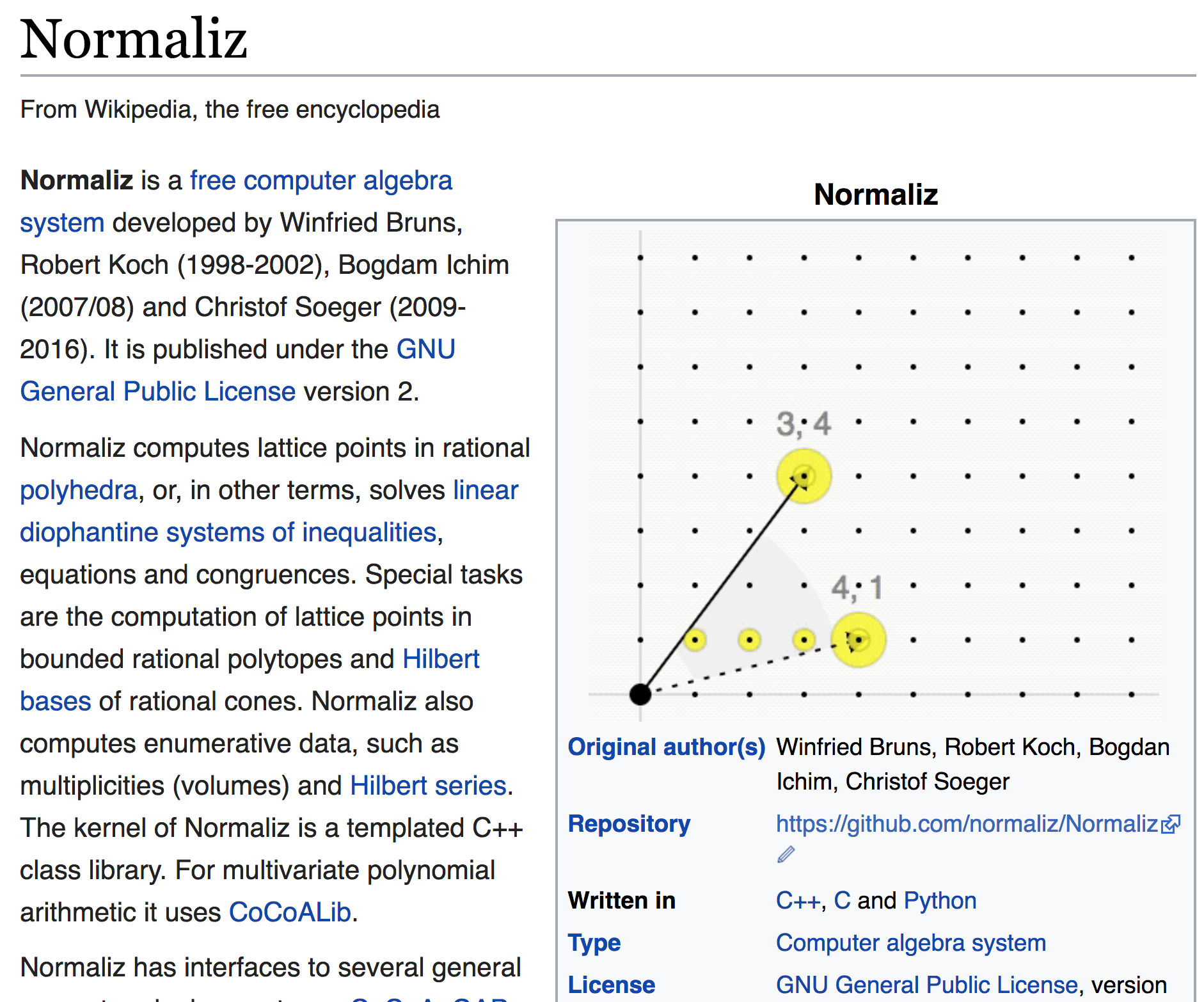
What is Normaliz?
Why a new computational backend?
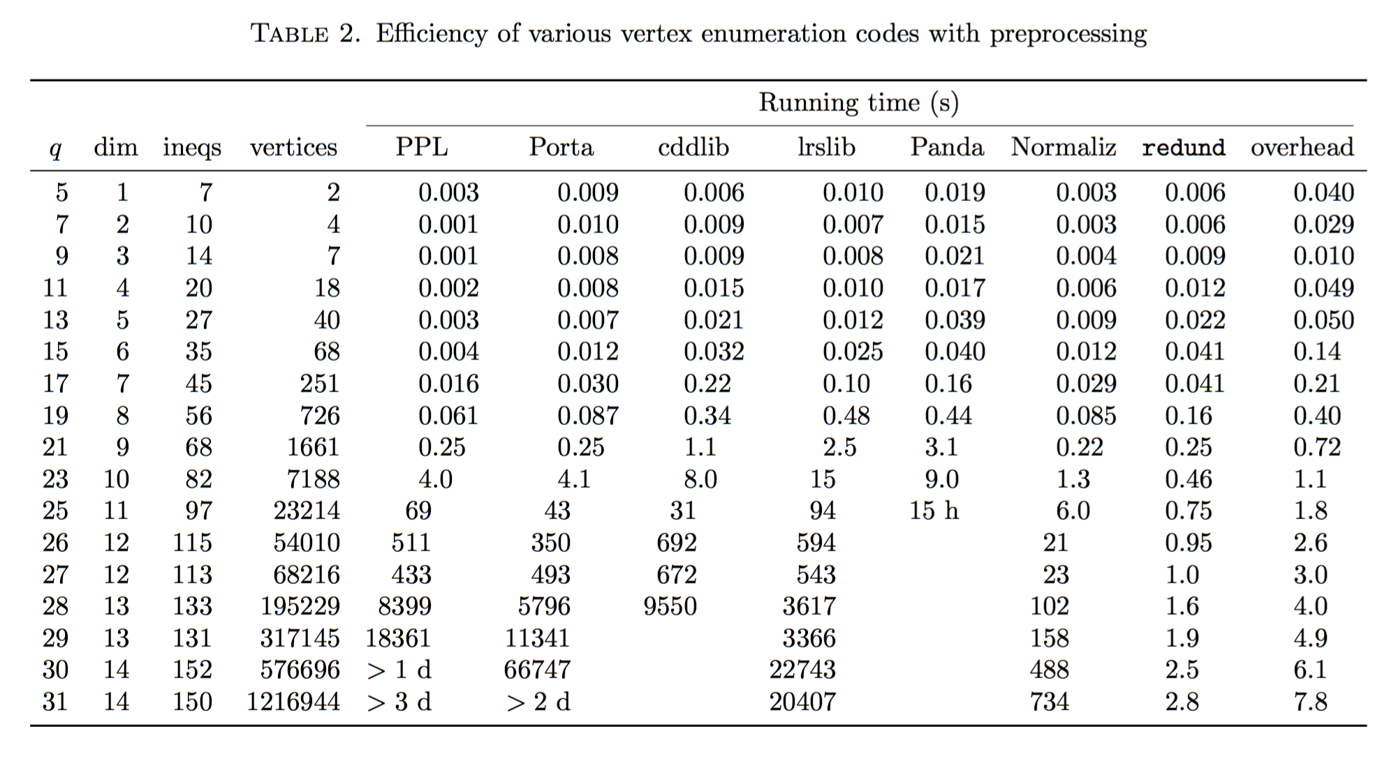
Performance matters.
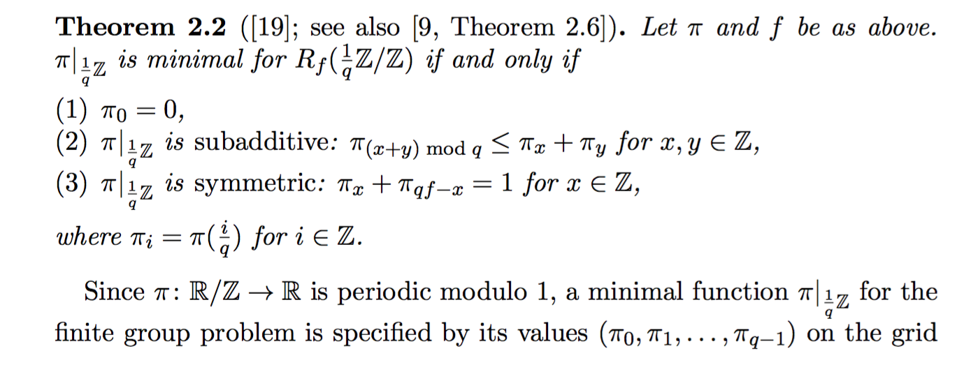
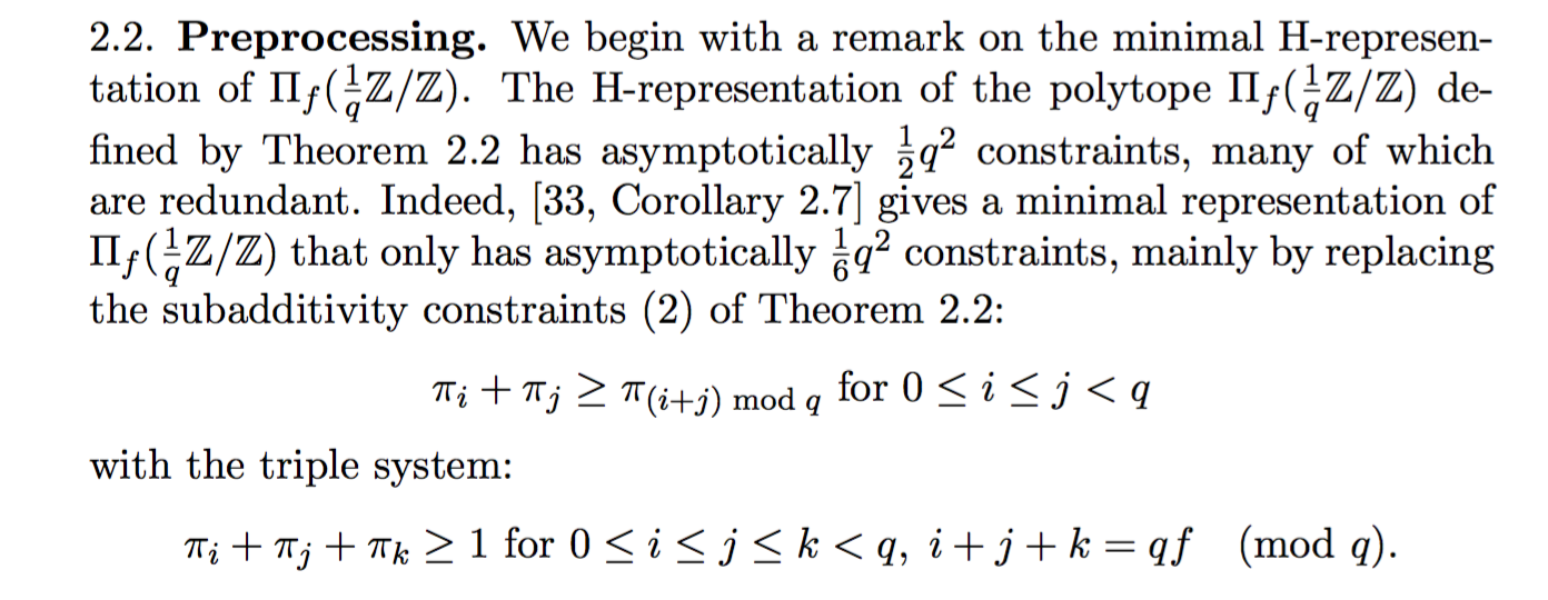
Case study: From the theory of subadditive functions
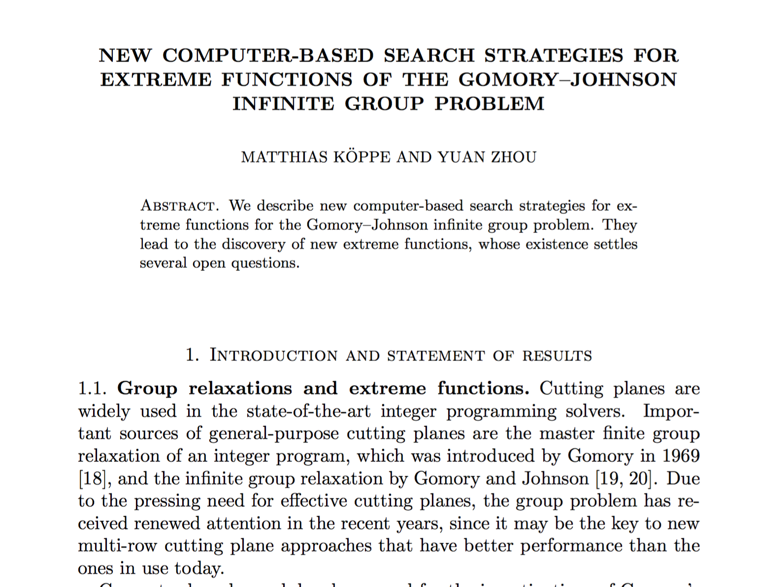
A family of polytopes with sparse inequalities, coefficients 1 and 2.
Wish to compute (and classify…) vertices
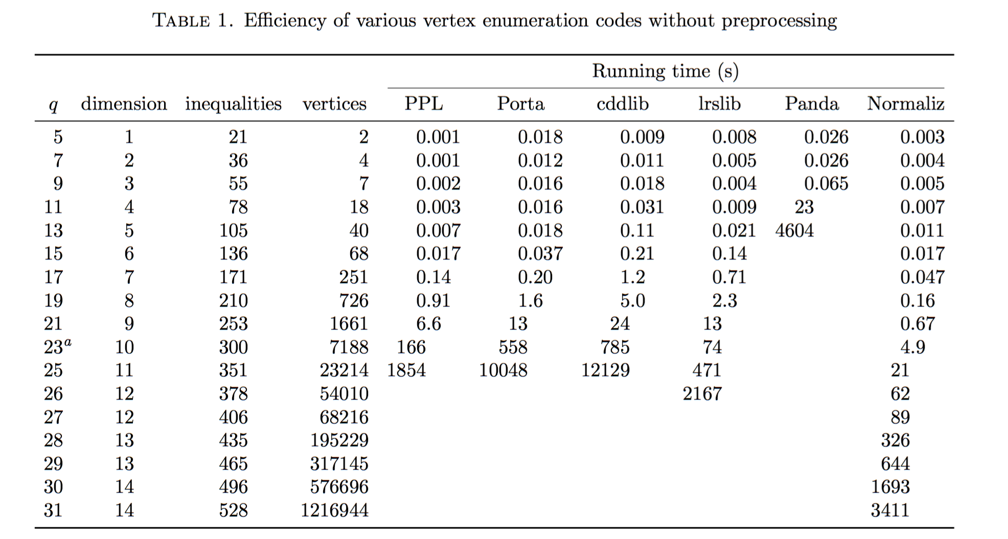
Could the problem be redundancy?
The normaliz backend
Optional SageMath packages:
normaliz (Bruns et al.)
Provides file-based command-line interface (not used in Sage) and a C++ API
PyNormaliz (Gutsche)
Install:
./sage -i pynormaliz
Python code: sage.geometry.polyhedron.backend_normaliz (Köppe)
sage: P1_normaliz = Polyhedron(vertices = [[1, 0], [0, 1]], rays = [[1, 1]], backend='normaliz')  # optional - pynormaliz
sage: type(P1_normaliz)                                                                           # optional - pynormaliz
<class 'sage.geometry.polyhedron.parent.Polyhedra_ZZ_normaliz_with_category.element_class'>
sage: P2_normaliz = Polyhedron(vertices = [[1/2, 0, 0], [0, 1/2, 0]],                             # optional - pynormaliz
....:                 rays = [[1, 1, 0]],
....:                 lines = [[0, 0, 1]], backend='normaliz')
sage: type(P2_normaliz)                                                                           # optional - pynormaliz
<class 'sage.geometry.polyhedron.parent.Polyhedra_QQ_normaliz_with_category.element_class'>
The backend normaliz provides other methods such as
integral_hull, which also works on unbounded polyhedra.
sage: P6 = Polyhedron(vertices = [[0, 0], [3/2, 0], [3/2, 3/2], [0, 3]], backend='normaliz')  # optional - pynormaliz
sage: IH = P6.integral_hull(); IH                                                             # optional - pynormaliz
A 2-dimensional polyhedron in QQ^2 defined as the convex hull of 4 vertices
sage: P1_normaliz.integral_hull()                                                             # optional - pynormaliz
A 2-dimensional polyhedron in ZZ^2 defined as the convex hull of 2 vertices and 1 ray
TODO: trac ticket #25091 - Make further computation goals of Normaliz available as methods.
New: polymake interface and polyhedral backend
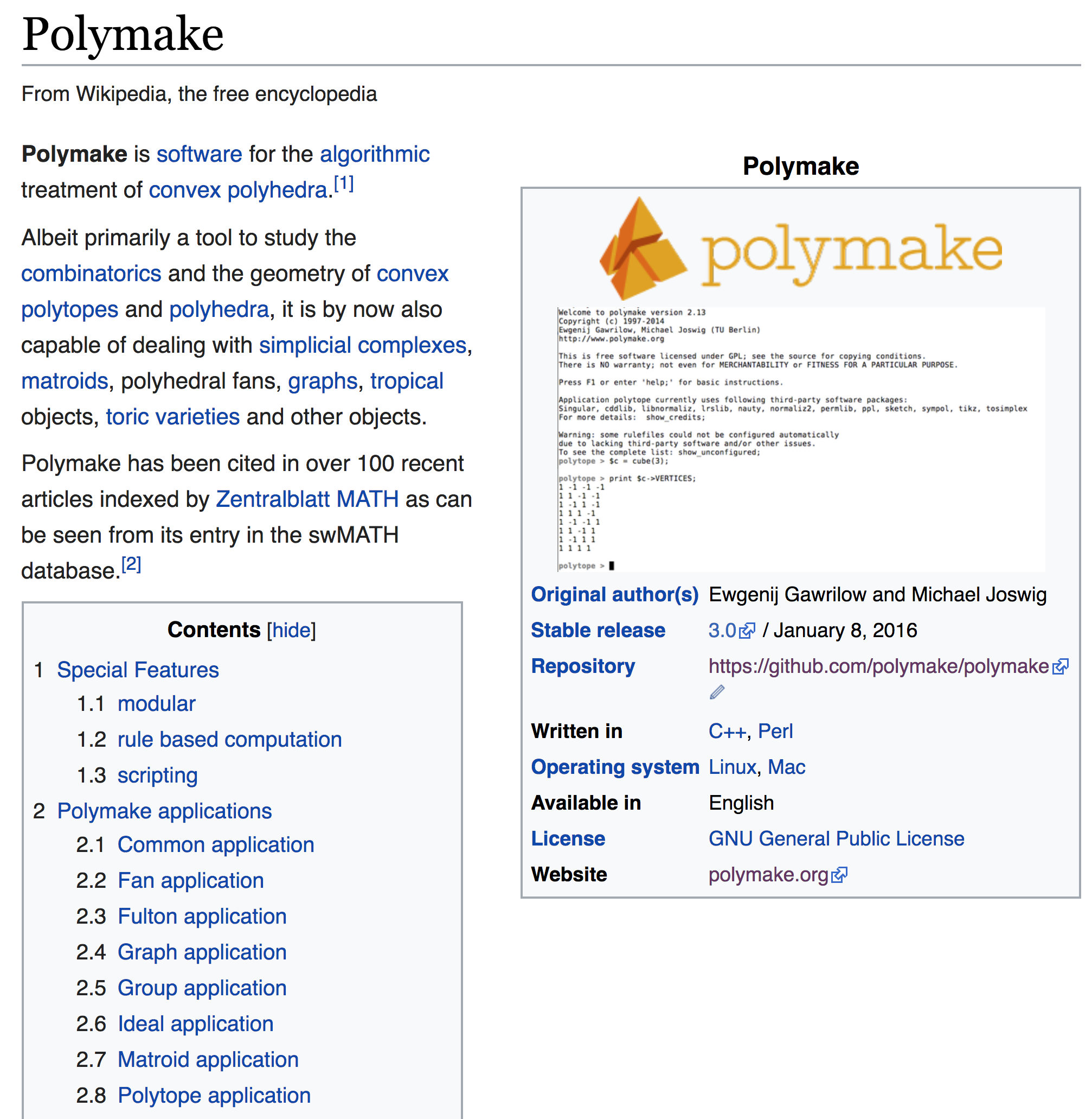
polymake interface in sage - sage.interfaces.polymake
Installation of polymake package for sage:
./sage -i polymake
polymake interface (a “pexpect” interface) developed by Simon King <simon.king@uni-jena.de> during the SageDays 84 in Olot (Spain).
Why use SageMath’s polymake interface instead of polymake directly
- Integration with the whole SageMath toolbox
- Programming languages: preferences, training
Another, ambitious effort to address the same problem

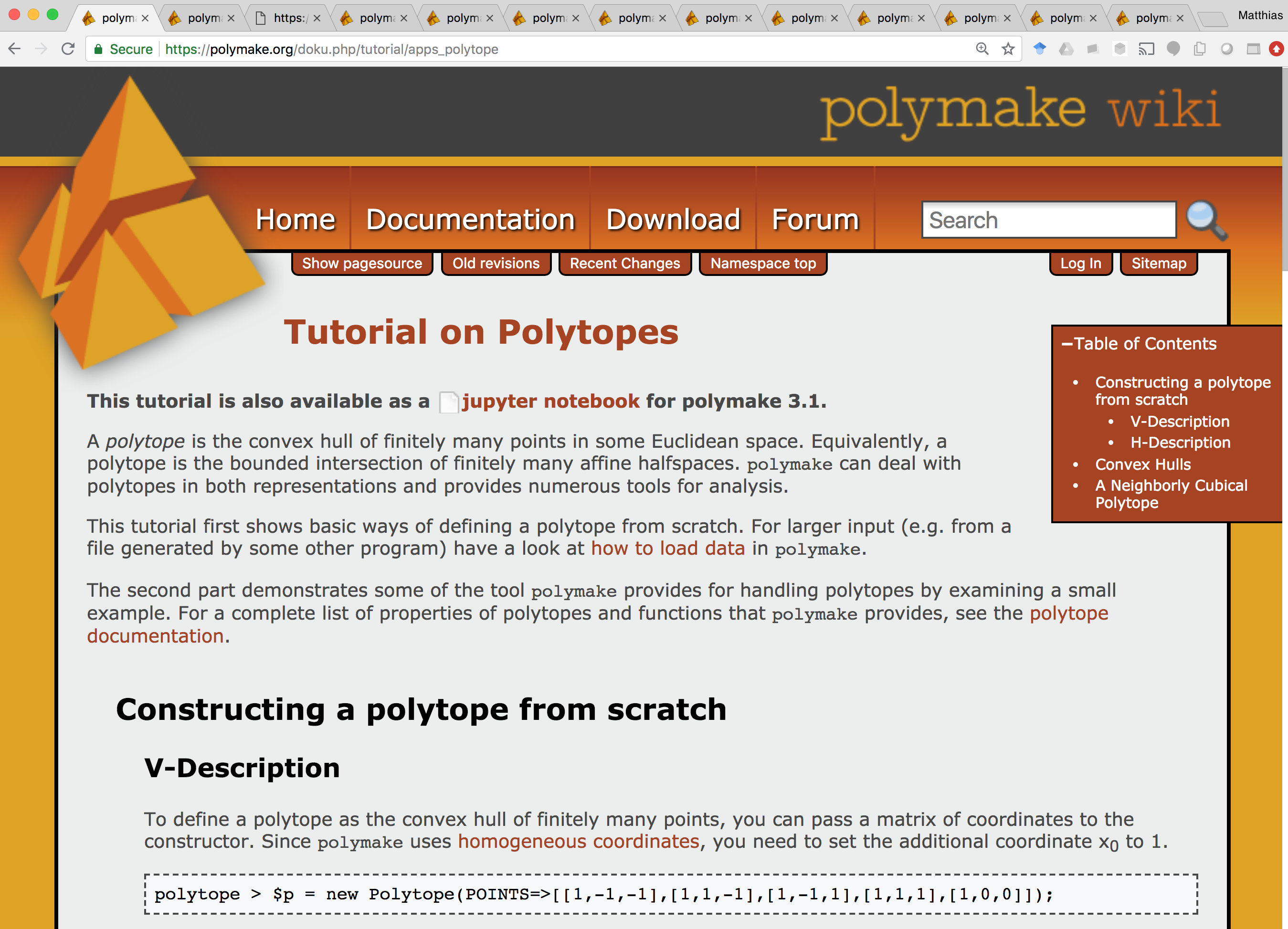
polymake tutorial on polytopes, translated to Python
Constructing a polytope from scratch
V-Description
To define a polytope as the convex hull of finitely many points, you can pass a matrix of coordinates to the constructor. Since polymake uses homogeneous coordinates, you need to set the additional coordinate x0 to 1.
polytope > $p = new Polytope(POINTS=>[[1,-1,-1],[1,1,-1],[1,-1,1],[1,1,1],[1,0,0]]);
In Sage:
sage: p = polymake.new_object("Polytope", POINTS=[[1,-1,-1],[1,1,-1],[1,-1,1],[1,1,1],[1,0,0]])
The result in SageMath is an interface object representing the Polymake object. It is not “converted”:
sage: p
Polytope<Rational>[SAGE43]
The POINTS can be any set of coordinates, they are not required to be irredundant nor vertices of their convex hull. To compute the actual vertices of our polytope, we do this:
polytope > print $p->VERTICES;
1 -1 -1
1 1 -1
1 -1 1
1 1 1
In Sage:
sage: p.VERTICES
1 -1 -1
1 1 -1
1 -1 1
1 1 1
What is this?
sage: V = _
sage: type(V)
<class 'sage.interfaces.polymake.PolymakeElement'>
Can convert to a Python list of interface elements:
sage: list(V)
[1 -1 -1, 1 1 -1, 1 -1 1, 1 1 1]
Or to a Python list of lists of Sage integers:
sage: [ list(ZZ(x) for x in v) for v in V ]
[[1, -1, -1], [1, 1, -1], [1, -1, 1], [1, 1, 1]]
Back to the polymake tutorial.
You can also add a lineality space via the input property INPUT_LINEALITY.
polytope > $p2 = new Polytope(POINTS=>[[1,-1,-1],[1,1,-1],[1,-1,1],[1,1,1],[1,0,0]],INPUT_LINEALITY=>[[0,1,0]]);
In Sage:
sage: p2 = polymake.new_object("Polytope", POINTS=[[1,-1,-1],[1,1,-1],[1,-1,1],[1,1,1],[1,0,0]], INPUT_LINEALITY=[[0,1,0]])
If you are sure that all the points really are extreme points (vertices) and your description of the lineality space is complete, you can define the polytope via the properties VERTICES and LINEALITY_SPACE instead of POINTS and INPUT_LINEALITY. This way, you can avoid unnecessary redundancy checks. The input properties POINTS / INPUT_LINEALITY may not be mixed with the properties VERTICES / LINEALITY_SPACE. Furthermore, the LINEALITY_SPACE must be specified as soon as the property VERTICES is used:
polytope > $p3 = new Polytope<Rational>(VERTICES=>[[1,-1,-1],[1,1,-1],[1,-1,1],[1,1,1]], LINEALITY_SPACE=>[]);
In Sage:
sage: p3 = polymake.new_object("Polytope<Rational>", VERTICES=[[1,-1,-1],[1,1,-1],[1,-1,1],[1,1,1]], LINEALITY_SPACE=[])
H-Description
It is also possible to define a polytope as an intersection of finitely many halfspaces, i.e., a matrix of inequalities. An inequality a0 + a1 x1 + … + ad xd >= 0 is encoded as a row vector (a0,a1,…,ad), see also Coordinates for Polyhedra. Here is an example:
polytope > $p4 = new Polytope(INEQUALITIES=>[[1,1,0],[1,0,1],[1,-1,0],[1,0,-1],[17,1,1]]);
In Sage:
p4 = polymake.new_object("Polytope", INEQUALITIES=[[1,1,0],[1,0,1],[1,-1,0],[1,0,-1],[17,1,1]])
The last inequality means 17+x1+x2 ≥ 0, hence it does not represent a facet of the polytope. If you want to take a look at the actual facets, do this:
polytope > print $p4->FACETS;
1 1 0
1 0 1
1 -1 0
1 0 -1
In Sage:
sage: p4.FACETS
If your polytope lies in an affine subspace then you can specify its equations via the input property EQUATIONS.
polytope > $p5 = new Polytope(INEQUALITIES=>[[1,1,0,0],[1,0,1,0],[1,-1,0,0],[1,0,-1,0]],EQUATIONS=>[[0,0,0,1],[0,0,0,2]]);
In Sage:
sage: p5 = polymake.new_object("Polytope", INEQUALITIES=[[1,1,0,0],[1,0,1,0],[1,-1,0,0],[1,0,-1,0]],EQUATIONS=[[0,0,0,1],[0,0,0,2]])
Again, if you are sure that all your inequalities are facets, you can use the properties FACETS and AFFINE_HULL instead. Note that this pair of properties is dual to the pair VERTICES / LINEALITY_SPACE described above.
Convex Hulls
Of course, polymake can convert the V-description of a polytope to its H-description and vice versa. Depending on the individual configuration polymake chooses one of the several convex hull computing algorithms that have a polymake interface. Available algorithms are double description (cdd of ppl), reverse search (lrs), and beneath beyond (internal). It is also possible to specify explicitly which method to use by using the prefer command:
polytope > prefer "lrs";                              # use lrs until revoked by another 'prefer' or 'reset_preference "lrs"'
polytope > $p = new Polytope(POINTS=>[[1,1],[1,0]]);

polytope > print $p->FACETS;
polymake: used package lrs
Implementation of the reverse search algorithm of Avis and Fukuda.
Copyright by David Avis.
http://cgm.cs.mcgill.ca/~avis/lrs.html
1 -1
0 1
In Sage:
sage: polymake.prefer('"lrs"') # Note double quoting to represent Perl strings
sage: p = polymake.new_object("Polytope", POINTS=[[1,1],[1,0]])
sage: p.FACETS
used package lrs
Implementation of the reverse search algorithm of Avis and Fukuda.
Copyright by David Avis.
http://cgm.cs.mcgill.ca/~avis/lrs.html
1 -1
0 1
sage: polymake.reset_preference('"lrs"')
100000004
A Neighborly Cubical Polytope
polymake provides a variety of standard polytope constructions and transformations. This example construction introduces some of them. Check out the documentation for a comprehensive list.
The goal is to construct a 4-dimensional cubical polytope which has the same graph as the 5-dimensional cube. It is an example of a neighborly cubical polytope as constructed in
Joswig & Ziegler: Neighborly cubical polytopes. Discrete Comput. Geom. 24 (2000), no. 2-3, 325–344, DOI 10.1007/s004540010039 This is the entire construction in a few lines of polymake code:
polytope > $c1 = cube(2);
polytope > $c2 = cube(2,2);
polytope > $p1x2 = product($c1,$c2);
polytope > $p2x1 = product($c2,$c1);
polytope > $nc = conv($p1x2,$p2x1);
In SageMath:
sage: c1 = polymake.cube(2)
sage: c2 = polymake.cube(2,2)
sage: p1x2 = polymake.product(c1, c2)
sage: p2x1 = polymake.product(c2, c1)
sage: nc = polymake.conv(p1x2, p2x1)
Let us examine more closely what this is about. First we constructed a square $c1 via calling the function cube. The only parameter 2 is the dimension of the cube to be constructed. It is not obvious how the coordinates are chosen; so let us check.
polytope > print $c1->VERTICES;
1 -1 -1
1 1 -1
1 -1 1
1 1 1
In SageMath:
sage: c1.VERTICES
1 -1 -1
1 1 -1
1 -1 1
1 1 1
The four vertices are listed line by line in homogeneous coordinates, where the homogenizing coordinate is the leading one. As shown the vertices correspond to the four choices of +/-1 in two positions. So the area of this square equals four, which is verified as follows:
polytope > print $c1->VOLUME;
4
In SageMath:
sage: c1.VOLUME
4
Here the volume is the Euclidean volume of the ambient space. Hence the volume of a polytope which is not full-dimensional is always zero. The second polytope $c2 constructed is also a square. However, the optional second parameter says that +/-2-coordinates are to be used rather than +/-1 as in the default case. The optional parameter is also allowed to be 0. In this case a cube with 0/1-coordinates is returned. You can access the documentation of functions by typing their name in the polymake shell and then hitting F1. The third command constructs the polytope $p1x2 as the cartesian product of the two squares. Clearly, this is a four-dimensional polytope which is combinatorially (even affinely) equivalent to a cube, but not congruent. This is easy to verify:
polytope > print isomorphic($p1x2,cube(4));
1
polytope > print congruent($p1x2,cube(4));
0
In SageMath:
sage: bool(polymake.isomorphic(p1x2,polymake.cube(4)))
True
sage: bool(polymake.congruent(p1x2,polymake.cube(4)))
False
Both return values are boolean, represented by the numbers 1 and 0, respectively. This questions are decided via a reduction to a graph isomorphism problem which in turn is solved via polymake’s interface to nauty. The polytope $p2x1 does not differ that much from the previous. In fact, the construction is twice the same, except for the ordering of the factors in the call of the function product. Let us compare the first vertices of the two products. One can see how the coordinates are induced by the ordering of the factors.
polytope > print $p1x2->VERTICES->[0];
1 -1 -1 -2 -2
polytope > print $p2x1->VERTICES->[0];
1 -2 -2 -1 -1
In SageMath:
sage: p1x2.VERTICES[0]
1 -1 -1 -2 -2
sage: p2x1.VERTICES[0]
1 -2 -2 -1 -1
In fact, one of these two products is obtained from the other by exchanging coordinate directions. Thats is to say, they are congruent but distinct as subsets of Euclidean 4-space. This is why taking their joint convex hull yields something interesting. Let us explore what kind of polytope we got.
A good idea then is to look at the f-vector. Beware, however, this usually requires to build the entire face lattice of the polytope, which is extremely costly. Therefore this is computationally infeasible for most high-dimensional polytopes.
polytope > print $nc->F_VECTOR;
32 80 72 24
In SageMath:
sage: nc.F_VECTOR
32 80 72 24
This is a first hint that our initial claim is indeed valid. The polytope constructed has 32 vertices and 80 = 32*5/2 edges, as many as the 5-dimensional cube:
polytope > print cube(5)->F_VECTOR;
32 80 80 40 10
In SageMath:
sage: polymake.cube(5).F_VECTOR
32 80 80 40 10
What is left is to check whether the vertex-edge graphs of the two polytopes actually are the same, and if all proper faces are combinatorially equivalent to cubes.
polytope > print isomorphic($nc->GRAPH->ADJACENCY,cube(5)->GRAPH->ADJACENCY);
1
polytope > print $nc->CUBICAL;
1
In SageMath:
sage: bool(polymake.isomorphic(nc.GRAPH.ADJACENCY, polymake.cube(5).GRAPH.ADJACENCY))
used package bliss
Computation of automorphism groups of graphs.
Copyright by Tommi Junttila and Petteri Kaski.
http://www.tcs.hut.fi/Software/bliss/
True
sage: bool(nc.CUBICAL)
True
See the tutorial on graphs for more on that subject.
The polymake backend
The polymake backend is provided when the experimental package polymake
for sage is installed.
sage: p = Polyhedron(vertices=[(0,0),(1,0),(0,1)],
....:                rays=[(1,1)], lines=[],
....:                backend='polymake', base_ring=QQ)
sage: p
A 2-dimensional polyhedron in QQ^2 defined as the convex hull of 3 vertices and 1 ray
Polyhedra with this backend are represented internally by a polymake interface object. We can get this interface object like this:
sage: polymake(p)
Polytope<Rational>[SAGE98]
TODO: Add Python methods to expose polymake computation goals (properties).
New: Polyhedra over algebraic number fields using QNormaliz
It is also possible to define polyhedra over algebraic numbers.
Why?
- Classic polyhedra
- Polyhedra with symmetries
- Number-theoretic applications
- Fast base case for semialgebraic computation? (Discuss.)
A classic SageMath feature - typical of CAS approach
A textbook implementation of the double description method in pure Python.
It works over general real fields, like AA, the algebraic reals.
sage: sqrt_2 = AA(2)^(1/2)
sage: cbrt_2 = AA(2)^(1/3)
sage: timeit('Polyhedron(vertices = [[sqrt_2, 0], [0, cbrt_2]])')  # random
5 loops, best of 3: 43.2 ms per loop
sage: P4 = Polyhedron(vertices = [[sqrt_2, 0], [0, cbrt_2]]); P4
A 1-dimensional polyhedron in AA^2 defined as the convex hull of 2 vertices
There is another way to create a polyhedron over algebraic numbers:
sage: K.<a> = NumberField(x^2 - 2, embedding=AA(2)**(1/2))
sage: L.<b> = NumberField(x^3 - 2, embedding=AA(2)**(1/3))
sage: timeit('Polyhedron(vertices = [[a, 0], [0, b]])')  # random
5 loops, best of 3: 39.9 ms per loop
sage: P5 = Polyhedron(vertices = [[a, 0], [0, b]]); P5
A 1-dimensional polyhedron in AA^2 defined as the convex hull of 2 vertices
If the base ring is known it may be a good option to use the proper sage.rings.number_field.number_field.number_field.composite_fields():
sage: J = K.composite_fields(L)[0]
sage: timeit('Polyhedron(vertices = [[J(a), 0], [0, J(b)]])')  # random
25 loops, best of 3: 9.8 ms per loop
sage: P5_comp = Polyhedron(vertices = [[J(a), 0], [0, J(b)]]); P5_comp
A 1-dimensional polyhedron in (Number Field in ab with defining polynomial x^6 - 6*x^4 - 4*x^3 + 12*x^2 - 24*x - 4)^2 defined as the convex hull of 2 vertices
Polymake
Polymake (and the sage backend for polymake) has support for algebraic polyhedra, but it is limited to quadratic fields:
sage: V = polytopes.dodecahedron().vertices_list()
sage: Polyhedron(vertices=V, backend='polymake')               # optional - polymake
A 3-dimensional polyhedron in (Number Field in sqrt5 with defining polynomial x^2 - 5)^3 defined as the convex hull of 20 vertices
Using Polymake’s internal implementation of the beneath-beyond method.
Our approach
(W. Bruns, V. Delecroix, S. Gutsche, M. Köppe, JP Labbe)
Take one of the best, actively developed and maintained polyhedral computation codes:
- Normaliz (Bruns et al.)
Suppress impulses such as:
- Fork the code
- “Because Python is such a clean language, we can just rewrite the whole thing in Python”
Instead: Convince upstream developer (Bruns) to generalize the code (without runtime cost; without source duplication (WIP)):
- QNormaliz (Bruns 2017-) - by using C++ templates, make parts of Normaliz code generic. Use a mock field (mpq_class) for prototyping
Prototype lower-level library for embedded number fields
- e-antic (Delecroix, 2016-),
building on state of the art libraries:
- arb (Johansson et al., 2013-),
- FLINT/ANTIC (Hart et al., 2013-).
Sage interfacing
- PyQNormaliz (Gutsche 2018),
- extended Sage backend_normaliz (Köppe 2018).
Status
Normaliz has QNormaliz/e-antic - stable release 3.6.3
Typical input file, normaliz/Qexample/dodecahedron-v.in:
amb_space 3
number_field min_poly (a^2 - 5) embedding [2.236067977499789 +/- 8.06e-16]
subspace 0
vertices 20
(-a + 3) (-a + 3) (-a + 3) 1
(2*a - 4) 0 (a - 1) 1
(-a + 3) (a - 3) (-a + 3) 1
(a - 1) (2*a - 4) 0 1
(a - 1) (-2*a + 4) 0 1
0 (a - 1) (2*a - 4) 1
0 (-a + 1) (2*a - 4) 1
(-2*a + 4) 0 (a - 1) 1
(a - 3) (-a + 3) (-a + 3) 1
(a - 3) (a - 3) (-a + 3) 1
(-a + 3) (-a + 3) (a - 3) 1
0 (a - 1) (-2*a + 4) 1
(-a + 3) (a - 3) (a - 3) 1
0 (-a + 1) (-2*a + 4) 1
(2*a - 4) 0 (-a + 1) 1
(-a + 1) (2*a - 4) 0 1
(-a + 1) (-2*a + 4) 0 1
(a - 3) (-a + 3) (a - 3) 1
(a - 3) (a - 3) (a - 3) 1
(-2*a + 4) 0 (-a + 1) 1
cone 0
Volume
Deg1Elements
IntegerHull
Sage interfacing: WIP at :trac:25097:
We need your algebraic polytopes
Thank you!