Normaliz’ed ANTICs: Polyhedral computation in an irrational (S)age
Matthias Köppe (UC Davis)
Talk at the IMA special workshop “SageMath and Macaulay2 - An Open Source Initiative”, 2019-07-24
Open source talk:
source:
$ git clone https://www.math.ucdavis.edu/~mkoeppe/art/ima-2019.gitLicense CC-BY-SA
based in part on SageMath tutorials
Contents and purpose of the talk:
- Introduction to SageMath
- Hands-on introduction to polyhedra, polyhedral computation, embedded algebraic number fields
- A tangent on recent software integration work in SageMath
- Report on a current implementation project for algebraic polyhedra
Quick introduction to SageMath
What is SageMath?
- “Python with mathematical batteries included”
- Python extended through its metaobject protocol by an object system driven by mathematical “categories” and “axioms”, similar to Axiom and Magma
- With less emphasis, also has general untyped symbolics (as needed in Calculus classes), provided by SymPy, Maxima, etc.
- Free software (GNU General Public License)
Two faces of SageMath:
sage-the-Python-library:
find src/sage -name "[a-z]*.py" -o -name "*.pyx" -o -name "*.pyd" | xargs wc -l

    263 src/sage/algebras/affine_nil_temperley_lieb.py
     38 src/sage/algebras/algebra.py
     69 src/sage/algebras/all.py
    343 src/sage/algebras/associated_graded.py
    110 src/sage/algebras/catalog.py
    326 src/sage/algebras/cellular_basis.py
   2840 src/sage/algebras/clifford_algebra.py
   2418 src/sage/algebras/cluster_algebra.py
   ...
    433 src/sage/geometry/polyhedron/backend_cdd.py
    268 src/sage/geometry/polyhedron/backend_field.py
    833 src/sage/geometry/polyhedron/backend_normaliz.py
    461 src/sage/geometry/polyhedron/backend_polymake.py
    266 src/sage/geometry/polyhedron/backend_ppl.py
   6970 src/sage/geometry/polyhedron/base.py
   ...
    340 src/sage/typeset/symbols.py
    161 src/sage/typeset/unicode_art.py
      5 src/sage/version.py
2163533 total
sage-the-software-distribution:
ls -1 build/pkgs/ && ls build/pkgs | wc -l

4ti2
alabaster
appnope
arb
atlas
...
polymake
polytopes_db
ppl
...
zlib
zn_poly
zope_interface
     286
Self-contained, just needs a compiler and build essentials to bootstrap (XCode command-line tools on macOS).
Installation:
Ignore binary distributions and source tarballs
Follow the instructions at http://doc.sagemath.org/html/en/developer/manual_git.html (“Git the hard way”) to checkout and build from source… or the following simplified instructions:
Check out most recent release:
$ git clone git://github.com/sagemath/sage.git
$ cd sage
$ git remote add trac git://trac.sagemath.org/sage.git
$ git remote set-url --push trac git@trac.sagemath.org:sage.git
$ git fetch trac master
$ git checkout master
Or, check out development version (current beta) - replace last two lines with
$ git fetch trac develop
$ git checkout develop
Build:
[user@localhost sage]$ MAKE='make -j8' make V=0
By tomorrow it will be finished
Optional steps that are useful for development (can do now, in a separate terminal, or later):
Create git worktrees (separate copies of the Sage sources, which share the repository with the main worktree). This allows you to work with several branches at the same time in a convenient way.
Use the main worktree (already created) as your “production copy” of Sage. You keep this at some release, or sometimes you will merge in branches (tickets) that you need for your work and that have not made it to a Sage release yet.
A worktree where you do development. You switch between branches and recompile often.
[user@localhost sage]$ git worktree add worktree-develop
cdinto the created folderworktree-develop, and build another copy of Sage there.[user@localhost sage]$ cd worktree-develop [user@localhost worktree-develop]$ ln -s ../upstream . # optional [user@localhost worktree-develop]$ MAKE='make -j8' make V=0
You now have two independent copies of the Sage source tree, and also two independent copies of the Sage installation (in the
localsubfolders).Another worktree that you only use for merging and rebasing tickets, not for compiling.
[user@localhost sage]$ git worktree add worktree-rebasing
Start it:
[user@localhost sage]$ ./sage
Then interact using the IPython REPL.
Other options:
- Ubuntu has sage packages
- Other Linux distros: https://repology.org/metapackage/sagemath/versions
- cocalc.com
- Docker images: sagemath, cocalc
- conda: http://doc.sagemath.org/html/en/installation/conda.html
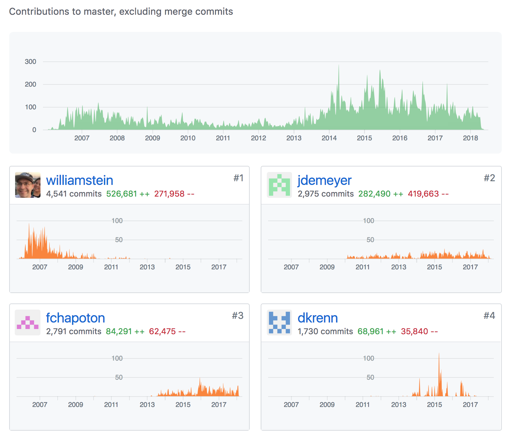
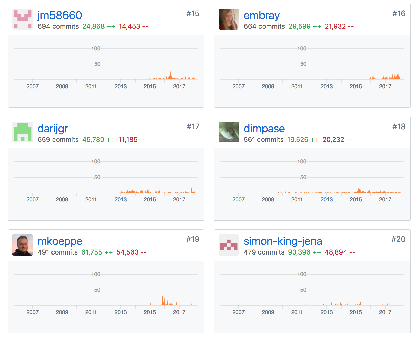
My contributions
- Some contributions to SageMath since 2015 (polyhedra,
optimization, build system)
scrolling down …
Change tickets at http://trac.sagemath.org with technical discussion
Tickets where I am an author of the code:
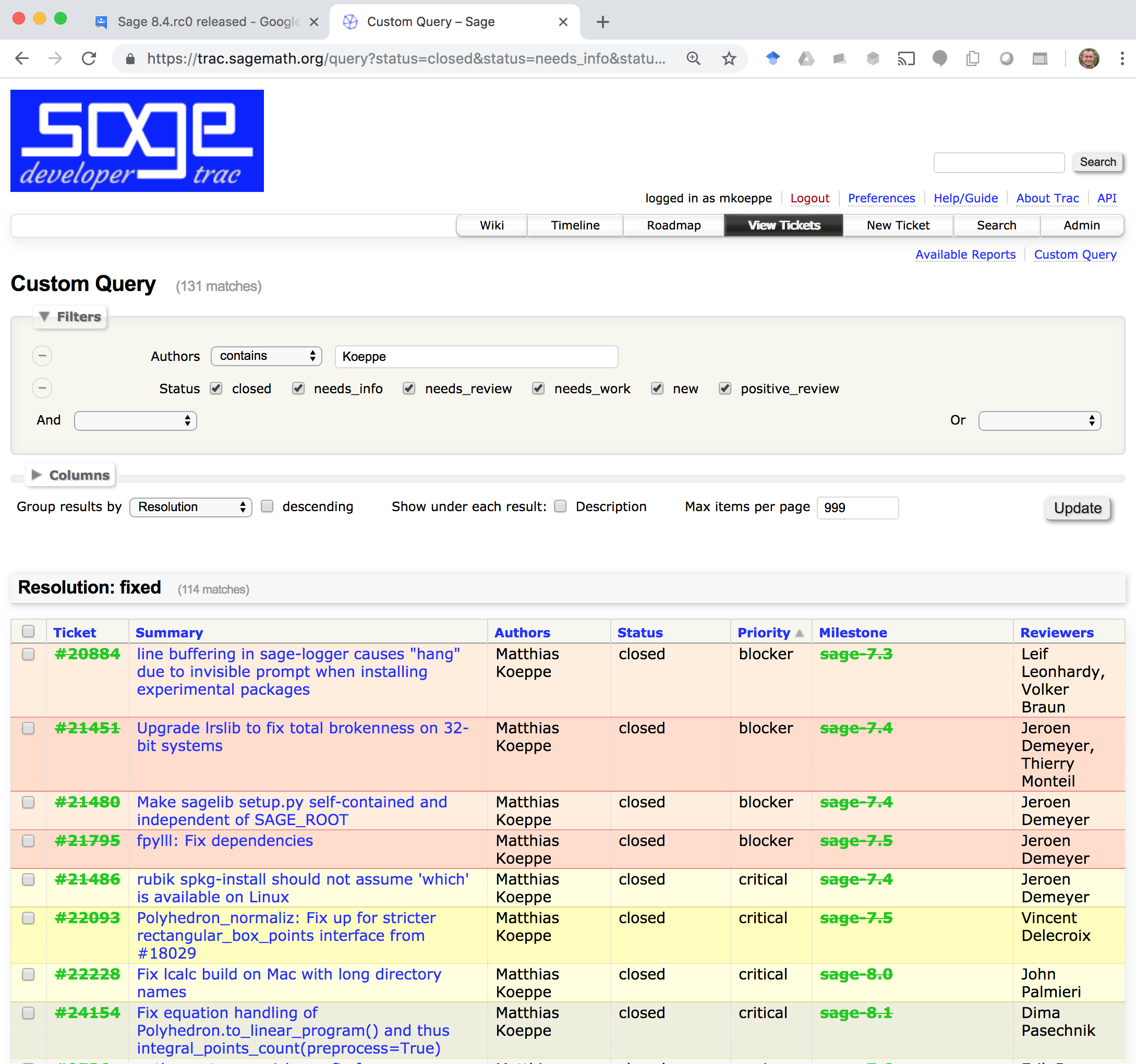
tickets I follow or have followed:
Metaticket:
- Meta-ticket: Polytopes, lattice (integer) point counting / enumeration, and their applications - https://trac.sagemath.org/ticket/20875
How to contribute to SageMath
- Log in to http://trac.sagemath.org with your GitHub account
- Create branch, make changes, build, run test suite, commit, create or update Trac ticket, push branch to ticket, set to “needs review”, wait for / find peer reviewer …
Introduction to polyhedra and the polyhedral computation facilities in SageMath
(Adapted from the tutorial “A Longer Introduction to Polyhedral Computations in Sage” in the SageMath documentation, written by Jean-Philippe Labbé <labbe@math.fu-berlin.de> during the SageDays 84 in Olot (Spain).)
Basic definitions and constructions
Given
- a real \((k\times d)\)-matrix \(A\), a real \((l\times d)\)-matrix \(C\),
- real vectors \(b\), \(d\) in \(\mathbb{R}^d\)
define a (convex) polyhedron \(P\) as the set of solutions of the system of linear inequalities:
- Each row of the system defines a closed half-space of \(\mathbb{R}^d\), or a hyperplane of \(\mathbb{R}^d\).
- Hence a polyhedron is the intersection of finitely many closed half-spaces in \(\mathbb{R}^d\).
This is an H-representation of the polyhedron \(P\).
- Minimal H-representations are “almost unique”:
- Inequalities are in bijection to facets
- Equations describe the affine hull of \(P\).
Farkas-Minkowski-Weyl Theorem:
Polyhedra are exactly those sets of \(\mathbb{R}^d\) that are finitely generated as follows:
\[x = \sum_{i=1}^{n}\lambda_iv_i+\sum_{i=1}^{m}\mu_ir_i + \sum_{i=1}^p \nu_i l_i,\]where
- \(v_i\) are fixed convex generators, \(\lambda_i\) convex multipliers,
- \(r_i\) are fixed conic generators, \(\mu_i\) conic multipliers,
- \(l_i\) are fixed linear generators, \(\nu_i\) linear multipliers.
This is a V-representation of the polyhedron \(P\).
Minimal V-representations are “almost unique”:
In the pointed case (lineality space of \(P\), maximal affine subspace \(L\) contained in \(P\), is trivial):
- \(v_i\) are vertices
- \(r_i\) are rays
- no \(l_i\).
Bounded case (no rays and no lines): a polytope.
\(V\)-representation
First, let’s define a polyhedron object as the convex hull of a set of points and some rays.
sage: P1 = Polyhedron(vertices = [[1, 0], [0, 1]], rays = [[1, 1]])
sage: P1
A 2-dimensional polyhedron in ZZ^2 defined as the convex hull of 2 vertices and 1 ray
The string representation already gives a lot of information:
- the dimension of the polyhedron (the smallest affine space containing it)
- the dimension of the space in which it is defined
- the base ring (\(\mathbb{Z}^2\)) over which the polyhedron lives (this specifies the parent class, see sage.geometry.polyhedron.parent)
- the number of vertices
- the number of rays
We can also add a lineality space.
sage: P2 = Polyhedron(vertices = [[1/2, 0, 0], [0, 1/2, 0]],
....:                 rays = [[1, 1, 0]],
....:                 lines = [[0, 0, 1]])
sage: P2
A 3-dimensional polyhedron in QQ^3 defined as the convex hull of 2 vertices, 1 ray, 1 line
\(H\)-representation
If a polyhedron object was constructed via a \(V\)-representation, Sage can provide the \(H\)-representation of the object.
sage: for h in P1.Hrepresentation():
....:     print(h)
An inequality (1, 1) x - 1 >= 0
An inequality (1, -1) x + 1 >= 0
An inequality (-1, 1) x + 1 >= 0
Each line gives a row of the matrix \(A\) and an entry of the vector \(b\).
The variable \(x\) is a vector in the ambient space where P1 is
defined. The \(H\)-representation may contain equations:
sage: P3.Hrepresentation()
(An inequality (-2.0, 0.0) x + 1.0 >= 0,
 An inequality (1.0, 0.0) x + 0.0 >= 0,
 An equation (1.0, 1.0) x - 0.5 == 0)
The construction of a polyhedron object via its \(H\)-representation,
requires a precise format. Each inequality \((a_{i1}, \dots, a_{id})\cdot
x + b_i \geq 0\) must be written as [b_i,a_i1, ..., a_id].
sage: P3_H = Polyhedron(ieqs = [[1.0, -2, 0], [0, 1, 0]], eqns = [[-0.5, 1, 1]])
sage: P3 == P3_H
True
sage: P3_H.Vrepresentation()
(A vertex at (0.0, 0.5), A vertex at (0.5, 0.0))
Representation objects
Many objects are related to the \(H\)- and \(V\)-representations. Sage has classes implemented for them.
\(H\)-representation
You can store the \(H\)-representation in a variable and use the inequalities and equalities as objects.
sage: P3_QQ = Polyhedron(vertices = [[0.5, 0], [0, 0.5]], base_ring=QQ)
sage: HRep = P3_QQ.Hrepresentation()
sage: H1 = HRep[0]; H1
An equation (2, 2) x - 1 == 0
sage: H2 = HRep[1]; H2
An inequality (0, -2) x + 1 >= 0
sage: H1.<tab>   # not tested
      H1.A                 H1.count             H1.incident          H1.is_H              H1.parent            H1.reset_name
      H1.adjacent          H1.dump              H1.index             H1.is_incident       H1.polyhedron        H1.save
      H1.b                 H1.dumps             H1.INEQUALITY        H1.is_inequality     H1.RAY               H1.type
      H1.category          H1.EQUATION          H1.interior_contains H1.LINE              H1.rename            H1.vector
      H1.contains          H1.eval              H1.is_equation       H1.neighbors         H1.repr_pretty       H1.VERTEX
sage: H1.A()
(2, 2)
sage: H1.b()
-1
sage: H1.is_equation()
True
sage: H1.is_inequality()
False
sage: H1.contains(vector([0,0]))
False
sage: H2.contains(vector([0,0]))
True
sage: H1.is_incident(H2)
True
It is possible to obtain the different objects of the \(H\)-representation as follows.
sage: P3_QQ.equations()
(An equation (2, 2) x - 1 == 0,)
sage: P3_QQ.inequalities()
(An inequality (0, -2) x + 1 >= 0, An inequality (0, 1) x + 0 >= 0)
Note
It is recommended to use equations or equation_generator
(and similarly for inequalities) if one wants to iterate over them instead
of equations_list.
\(V\)-representation
Similarly, you can access vertices, rays and lines of the polyhedron.
sage: VRep = P2.Vrepresentation(); VRep
(A line in the direction (0, 0, 1),
 A vertex at (0, 1/2, 0),
 A vertex at (1/2, 0, 0),
 A ray in the direction (1, 1, 0))
sage: L = VRep[0]; L
A line in the direction (0, 0, 1)
sage: V = VRep[1]; V
A vertex at (0, 1/2, 0)
sage: R = VRep[3]; R
A ray in the direction (1, 1, 0)
sage: L.is_line()
True
sage: L.is_incident(V)
True
sage: R.is_incident(L)
False
sage: L.vector()
(0, 0, 1)
sage: V.vector()
(0, 1/2, 0)
It is possible to obtain the different objects of the \(V\)-representation as follows.
sage: P2.vertices()
(A vertex at (0, 1/2, 0), A vertex at (1/2, 0, 0))
sage: P2.rays()
(A ray in the direction (1, 1, 0),)
sage: P2.lines()
(A line in the direction (0, 0, 1),)

sage: P2.vertices_matrix()
[  0 1/2]
[1/2   0]
[  0   0]
Note
It is recommended to use vertices or vertex_generator
(and similarly for rays and lines) if one wants to iterate over them instead
of vertices_list.
How does SageMath convert between V- and H-representation?
It knows how to do this,
- sage.geometry.polyhedron.backend_field (a pure Python implementation)
but, if possible, it prefers to delegate it to a library that knows better
sage.geometry.polyhedron.backend_cdd
- cddlib by Fukuda (1999-); see The cdd and cddplus homepage
sage.geometry.polyhedron.backend_ppl
- Parma Polyhedra Library by Bagnara et al., 2001-; see The Parma Polyhedra Library homepage
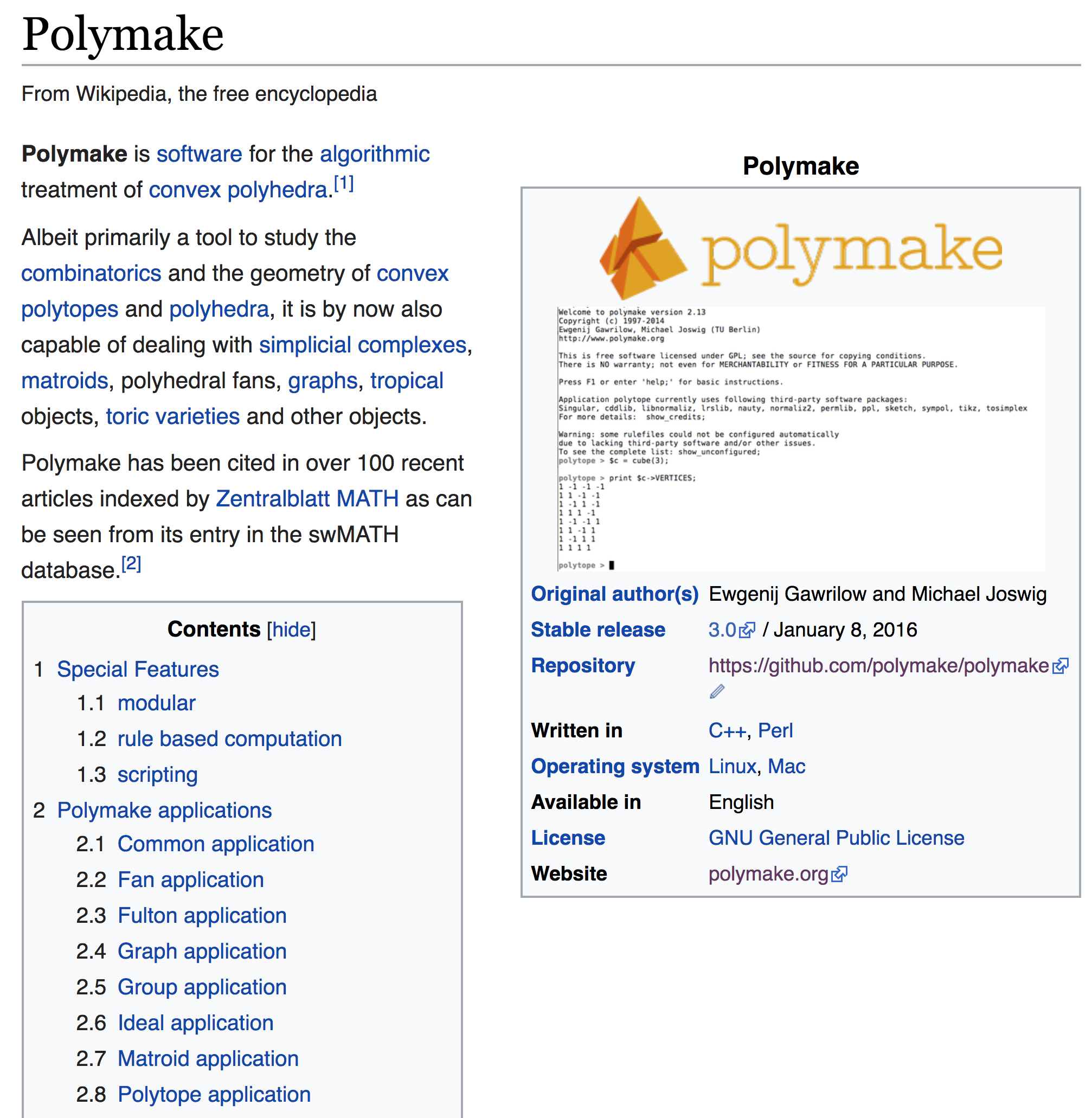
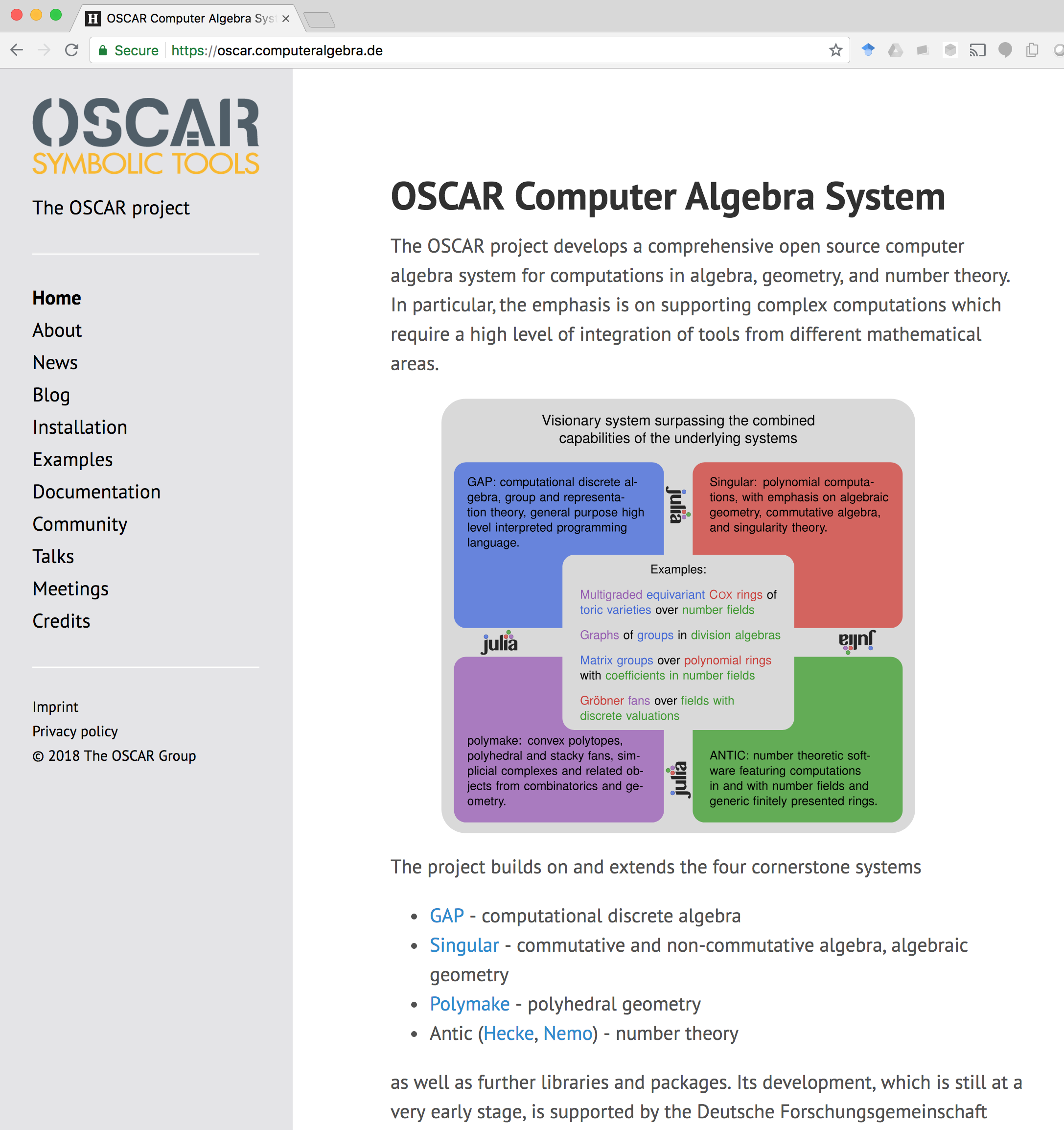
sage.geometry.polyhedron.backend_polymake,
The polymake project for convex geometry, by Gawrilow, Joswig, et al. 1997-
requires the optional SageMath package
polymake:$ sage -i polymakesage.geometry.polyhedron.backend_normaliz, (requires the optional package
pynormaliz)
- Normaliz by Bruns et al., 1998-
Really, how does it do this?
Let’s convert from V to H, and let’s assume the compact case (polytope).
The finite generation description of \(P\):
is a polyhedron \(Q\) (in variables \(x\) and \(\lambda\)), an extended formulation of \(P\). \(P\) is the projection of \(Q\) to space of \(x\) variables.
First eliminate the equations by pivoting (Gaussian elimination).
Then project out the remaining \(\lambda_i\) variables using Fourier-Motzkin elimination… worst-case quadratic blow-up for each variable.
Variants: Double description method; beneath-beyond method
Alternative algorithm based on pivoting: lexicographic reverse search (lrslib, Avis et al., 2000-)
Backends for polyhedral computations
To deal with polyhedron objects, Sage has several backends available.
The cdd backend
In order to use a specific backend, we specify the backend parameter.
sage: P1_cdd = Polyhedron(vertices = [[1, 0], [0, 1]], rays = [[1, 1]], backend='cdd')
sage: P1_cdd
A 2-dimensional polyhedron in QQ^2 defined as the convex hull of 2 vertices and 1 ray
The cdd backend accepts also entries in RDF (double
precision floating point numbers):
sage: P3_cdd = Polyhedron(vertices = [[0.5, 0], [0, 0.5]], backend='cdd')
sage: P3_cdd
A 1-dimensional polyhedron in RDF^2 defined as the convex hull of 2 vertices
The ppl backend
The default backend for polyhedron objects is ppl.
sage: type(P1)
<class 'sage.geometry.polyhedron.parent.Polyhedra_ZZ_ppl_with_category.element_class'>
sage: type(P2)
<class 'sage.geometry.polyhedron.parent.Polyhedra_QQ_ppl_with_category.element_class'>
sage: type(P3)  # has entries like 0.5
<class 'sage.geometry.polyhedron.parent.Polyhedra_RDF_cdd_with_category.element_class'>
As you see, it does not accepts values in RDF and the polyhedron constructor
used the cdd backend.
Methods of polyhedra
sage: p = Polyhedron()
sage: p.<tab>             # not tested
      p.adjacency_matrix                 p.facet_adjacency_matrix           p.lattice_polytope                 p.rays_list
      p.affine_hull                      p.gale_transform                   p.line_generator                   p.relative_interior_contains
      p.ambient_dim                      p.get_integral_point               p.lines                            p.rename
      p.ambient_space                    p.graph                            p.lines_list                       p.render_solid
      p.backend                          p.Hrep_generator                   p.minkowski_difference             p.render_wireframe
      p.barycentric_subdivision          p.Hrepresentation                  p.Minkowski_difference             p.repr_pretty_Hrepresentation
      p.base_extend                      p.Hrepresentation_space            p.minkowski_sum                    p.representative_point
      p.base_ring                        p.Hrepresentation_str              p.Minkowski_sum                    p.reset_name
      p.bipyramid                        p.hyperplane_arrangement           p.n                                p.restricted_automorphism_group
      p.bounded_edges                    p.incidence_matrix                 p.N                                p.save
      p.bounding_box                     p.inequalities                     p.n_equations                      p.schlegel_projection
      p.cartesian_product                p.inequalities_list                p.n_facets                         p.show
      p.category                         p.inequality_generator             p.n_Hrepresentation                p.stack
      p.cdd_Hrepresentation              p.integral_points                  p.n_inequalities                   p.subdirect_sum
      p.cdd_Vrepresentation              p.integral_points_count            p.n_lines                          p.subs
      p.center                           p.integrate                        p.n_rays                           p.substitute
      p.combinatorial_automorphism_group p.interior_contains                p.n_vertices                       p.to_linear_program
      p.contains                         p.intersection                     p.n_Vrepresentation                p.translation
      p.convex_hull                      p.is_combinatorially_isomorphic    p.neighborliness                   p.triangulate
      p.dilation                         p.is_compact                       p.normal_fan                       p.truncation
      p.dim                              p.is_empty                         p.numerical_approx                 p.vertex_adjacency_matrix
      p.dimension                        p.is_full_dimensional              p.one_point_suspension             p.vertex_digraph
      p.direct_sum                       p.is_idempotent                    p.parent                           p.vertex_facet_graph
      p.dump                             p.is_inscribed                     p.plot                             p.vertex_generator
      p.dumps                            p.is_lattice_polytope              p.polar                            p.vertex_graph
      p.equation_generator               p.is_minkowski_summand             p.prism                            p.vertices
      p.equations                        p.is_Minkowski_summand             p.product                          p.vertices_list
      p.equations_list                   p.is_neighborly                    p.projection                       p.vertices_matrix
      p.f_vector                         p.is_simple                        p.pyramid                          p.volume
      p.face_fan                         p.is_simplex                       p.radius                           p.Vrep_generator
      p.face_lattice                     p.is_simplicial                    p.radius_square                    p.Vrepresentation
      p.face_split                       p.is_universe                      p.random_integral_point            p.Vrepresentation_space
      p.face_truncation                  p.is_zero                          p.ray_generator                    p.write_cdd_Hrepresentation
      p.faces                            p.join                             p.rays                             p.write_cdd_Vrepresentation
Polyhedra over algebraic number fields
(with W. Bruns, V.~Delecroix, S.~Gutsche, J.-P.~Labb’e)
We want to do exact computations over non-rational polyhedra.
Why?
- Classic polyhedra
- Polyhedra with symmetries
- Combinatorial types of polyhedra that cannot be realized using rationals (Perles)
- Number-theoretic applications
- Fast base case for semialgebraic computation
The classic polyhedra: A first example
The regular icosahedron has 20 regular triangles as facets.
SageMath includes a nice library of polytopes that has a constructor for the icosahedron.
Let’s look at the (simplified) source code.
sage: polytopes.icosahedron??
Signature: polytopes.icosahedron(exact=True, base_ring=None, backend=None)
Source:
    def icosahedron(self, exact=True, base_ring=None, backend=None):
        r"""
        Return an icosahedron with edge length 1.

        The icosahedron is one of the Platonic solid. It has 20 faces
        and is dual to the :meth:`dodecahedron`.

        INPUT:

        - ``exact`` -- (boolean, default ``True``) If ``False`` use an
          approximate ring for the coordinates.

        - ``base_ring`` -- (optional) the ring in which the coordinates will
          belong to.  Note that this ring must contain `\sqrt(5)`. If it is not
          provided and ``exact=True`` it will be the number field
          `\QQ[\sqrt(5)]` and if ``exact=False`` it will be the real double
          field.

        - ``backend`` -- the backend to use to create the polytope.

        ...

        """
        ... g = (1 + base_ring(5).sqrt()) / 2
        r12 = base_ring.one() / 2
        z = base_ring.zero()
        pts = [[z, s1 * r12, s2 * g / 2]
               for s1, s2 in itertools.product([1, -1], repeat=2)]
        verts = [p(v) for p in AlternatingGroup(3) for v in pts]
        return Polyhedron(vertices=verts, base_ring=base_ring, backend=backend)
File:      ...sage/geometry/polyhedron/library.py
Type:      instancemethod
The regular icosahedron cannot be realized with rational coordinates. \(\sqrt5\) necessarily appears.
Let’s try to construct a number field \(\QQ(\sqrt5)\) for this.
sage: x = polygen(QQ, 'x')
sage: K = NumberField(x^2 - 5, 'a')
sage: a = K.gen()
sage: a.minpoly()
x^2 - 5
sage: a^2
5
Looking good. But…
sage: CC(a)
TypeError: unable to coerce to a ComplexNumber: <type 'sage.rings.number_field.number_field_element_quadratic.NumberFieldElement_quadratic'>
It is the abstract number field \(\QQ(a)\) with \(a^2 = 5\). It does not know the embedding of the generator \(a\) into the real or complex numbers.
In order to define polyhedra, we need a real field so that inequalities make sense.
sage: x = polygen(QQ, 'x')
sage: K = NumberField(x^2 - 5, 'a', embedding=2.0)
sage: a = K.gen()
Here 2.0 is a coarse approximation of \(\sqrt{5}\). It is good enough to select the intended positive root.
sage: RR(a)
2.23606797749979
Success!
But are we now back to inexact floating point computation?
No:
All arithmetic is done in rational arithmetic using the coordinates in the power basis of \(a\)
Comparing two numbers for equality uses the rational coordinates
Comparing two numbers regarding their real embeddings:
Special code for quadratic field extensions:
If \(a \geq c\) and \(b \leq d\), then
\[ \begin{align}\begin{aligned}a + b \sqrt{5} > c + d \sqrt{5}\\\iff (a - c)^2 > (d - b)^2 5\end{aligned}\end{align} \]For general absolute field extensions, use interval arithmetic for rigorous root refinement, by bisection and Newton’s method.
Let’s set up the icosahedron using this field.
sage: P = polytopes.icosahedron(base_ring=K)
sage: P
A 3-dimensional polyhedron in (Number Field in a with defining polynomial x^2 - 5)^3 defined as the convex hull of 12 vertices
We can query its V- and H-representation.
sage: P.vertices()
(A vertex at (0, 1/2, 1/4*a + 1/4),
 A vertex at (0, -1/2, 1/4*a + 1/4),
 A vertex at (1/2, 1/4*a + 1/4, 0),
 A vertex at (1/2, -1/4*a - 1/4, 0),
 A vertex at (1/4*a + 1/4, 0, 1/2),
 A vertex at (1/4*a + 1/4, 0, -1/2),
 A vertex at (-1/2, 1/4*a + 1/4, 0),
 A vertex at (-1/2, -1/4*a - 1/4, 0),
 A vertex at (-1/4*a - 1/4, 0, 1/2),
 A vertex at (0, 1/2, -1/4*a - 1/4),
 A vertex at (0, -1/2, -1/4*a - 1/4),
 A vertex at (-1/4*a - 1/4, 0, -1/2))
sage: P.inequalities()
(An inequality (0, -1, 1/2*a - 3/2) x + 1/4*a + 1/4 >= 0,
 An inequality (0, -1, -1/2*a + 3/2) x + 1/4*a + 1/4 >= 0,
 An inequality (0, 1, 1/2*a - 3/2) x + 1/4*a + 1/4 >= 0,
 An inequality (0, 1, -1/2*a + 3/2) x + 1/4*a + 1/4 >= 0,
 An inequality (-1/2*a + 1/2, -1/2*a + 1/2, -1/2*a + 1/2) x + 1/4*a + 1/4 >= 0,
 An inequality (1/2*a - 3/2, 0, -1) x + 1/4*a + 1/4 >= 0,
 An inequality (-1/2*a + 1/2, 1/2*a - 1/2, -1/2*a + 1/2) x + 1/4*a + 1/4 >= 0,
 An inequality (1/2*a - 1/2, -1/2*a + 1/2, -1/2*a + 1/2) x + 1/4*a + 1/4 >= 0,
 An inequality (1/2*a - 1/2, 1/2*a - 1/2, -1/2*a + 1/2) x + 1/4*a + 1/4 >= 0,
 An inequality (-1/2*a + 3/2, 0, -1) x + 1/4*a + 1/4 >= 0,
 An inequality (-1/2*a + 1/2, -1/2*a + 1/2, 1/2*a - 1/2) x + 1/4*a + 1/4 >= 0,
 An inequality (-1/2*a + 1/2, 1/2*a - 1/2, 1/2*a - 1/2) x + 1/4*a + 1/4 >= 0,
 An inequality (-1, 1/2*a - 3/2, 0) x + 1/4*a + 1/4 >= 0,
 An inequality (-1, -1/2*a + 3/2, 0) x + 1/4*a + 1/4 >= 0,
 An inequality (1/2*a - 3/2, 0, 1) x + 1/4*a + 1/4 >= 0,
 An inequality (1/2*a - 1/2, -1/2*a + 1/2, 1/2*a - 1/2) x + 1/4*a + 1/4 >= 0,
 An inequality (1/2*a - 1/2, 1/2*a - 1/2, 1/2*a - 1/2) x + 1/4*a + 1/4 >= 0,
 An inequality (1, 1/2*a - 3/2, 0) x + 1/4*a + 1/4 >= 0,
 An inequality (1, -1/2*a + 3/2, 0) x + 1/4*a + 1/4 >= 0,
 An inequality (-1/2*a + 3/2, 0, 1) x + 1/4*a + 1/4 >= 0)
And combinatorial data.
sage: P.f_vector()
(1, 12, 30, 20, 1)
Who did this computation?
sage: P.backend()
'field'
OK, that’s bad news. We are paying two performance penalties here.
sage: %timeit polytopes.hypercube(6, backend='ppl')    # random
100 loops, best of 3: 8.2 ms per loop

sage: vertices_QQ = polytopes.hypercube(6, backend='ppl').base_extend(QQ).vertices_list()
sage: %timeit Polyhedron(vertices=vertices_QQ, backend='field')    # random
1 loop, best of 3: 1.7 s per loop

sage: vertices_Q5 = polytopes.hypercube(6, backend='ppl').base_extend(QuadraticField(5)).vertices_list()
sage: %timeit Polyhedron(vertices=vertices_Q5, backend='field')
10 loops, best of 3: 125 ms per loop

sage: vertices_AA = polytopes.hypercube(6, backend='ppl').base_extend(AA).vertices_list()
sage: %timeit Polyhedron(vertices=vertices_AA, backend='field')
1 loop, best of 3: 2.18 s per loop
New: polymake interface and polyhedral backend
polymake interface in sage - sage.interfaces.polymake
Installation of polymake package for sage:
./sage -i polymake
polymake interface (a “pexpect” interface) developed by Simon King <simon.king@uni-jena.de> during the SageDays 84 in Olot (Spain).
Why use SageMath’s polymake interface instead of polymake directly
- Integration with the whole SageMath toolbox
- Programming languages: preferences, training
Another, ambitious effort to address the same problem
The polymake backend
The polymake backend is provided when the experimental package polymake
for sage is installed.
sage: p = Polyhedron(vertices=[(0,0),(1,0),(0,1)],
....:                rays=[(1,1)], lines=[],
....:                backend='polymake', base_ring=QQ)
sage: p
A 2-dimensional polyhedron in QQ^2 defined as the convex hull of 3 vertices and 1 ray
Polyhedra with this backend are represented internally by a polymake interface object. We can get this interface object like this:
sage: polymake(p)
Polytope<Rational>[SAGE98]
TODO: Add Python methods to expose polymake computation goals (properties).
Polyhedra over quadratic fields with Polymake
Polymake (and the sage backend for polymake) has support for algebraic polyhedra, but it is limited to quadratic fields:
sage: V = polytopes.dodecahedron().vertices_list()
sage: Polyhedron(vertices=V, backend='polymake')               # optional - polymake
A 3-dimensional polyhedron in (Number Field in sqrt5 with defining polynomial x^2 - 5)^3 defined as the convex hull of 20 vertices
Using Polymake’s internal implementation of the beneath-beyond method.
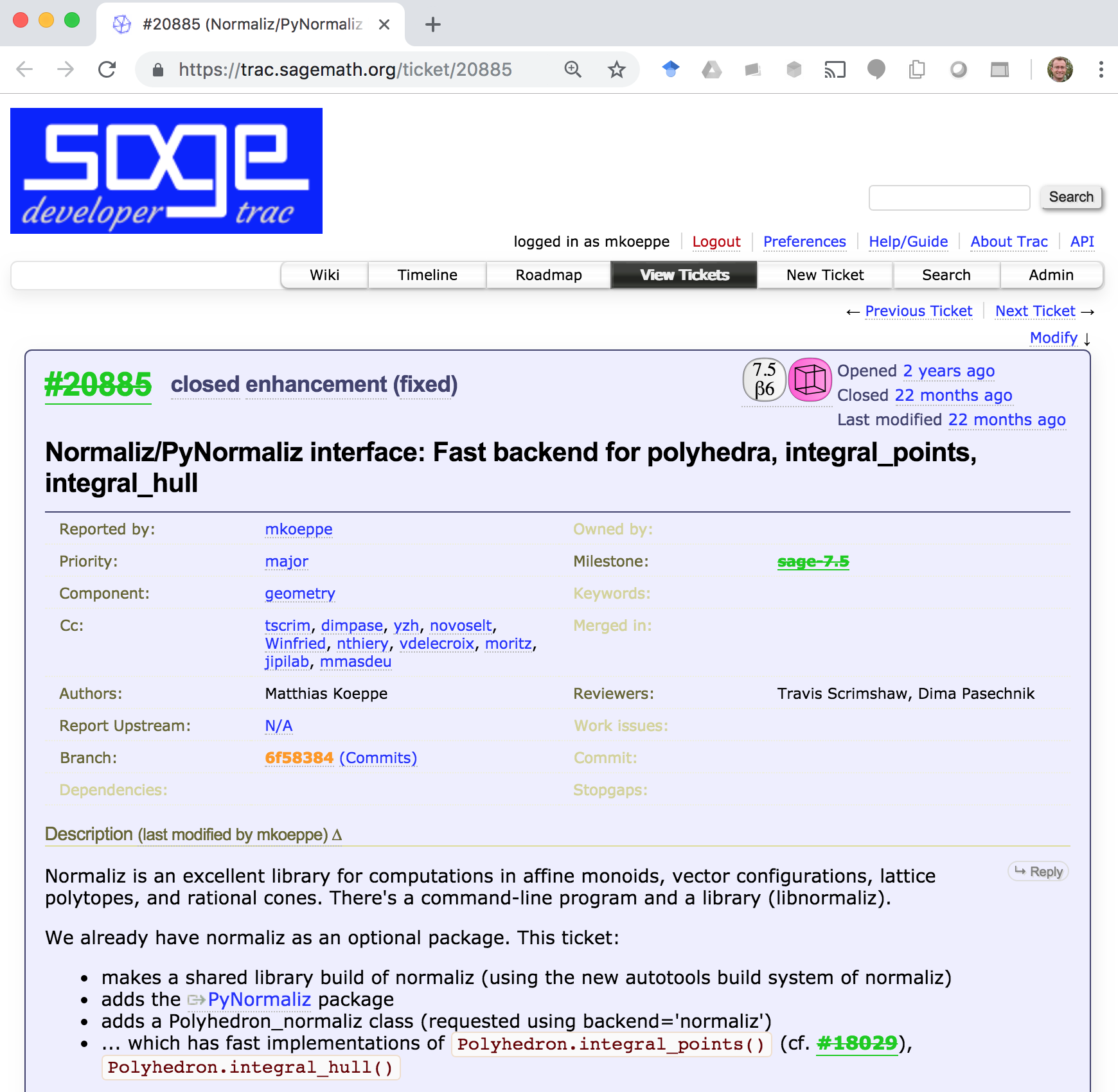
New: computational backend using Normaliz
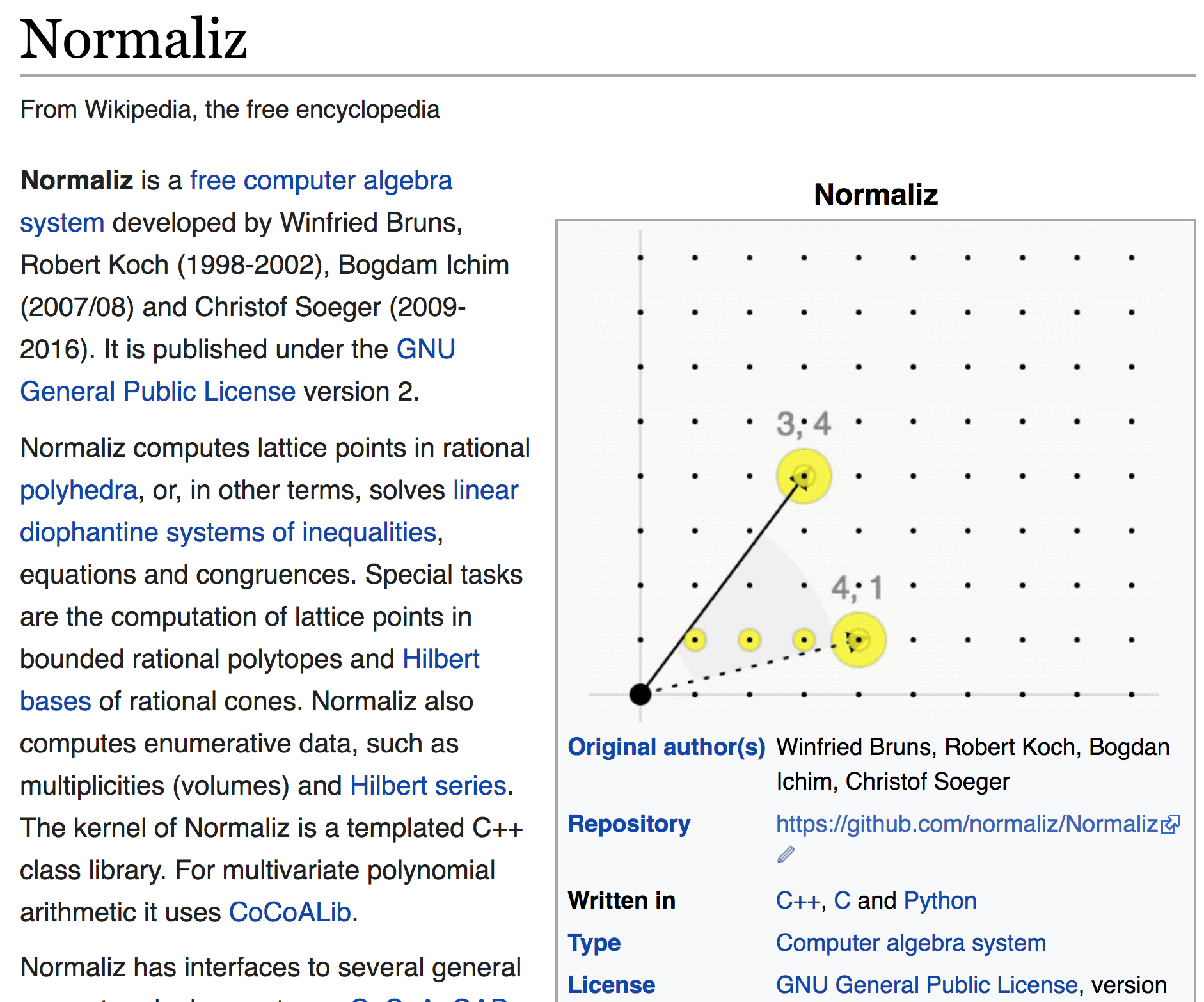
What is Normaliz?
Why a new computational backend?
Performance matters.
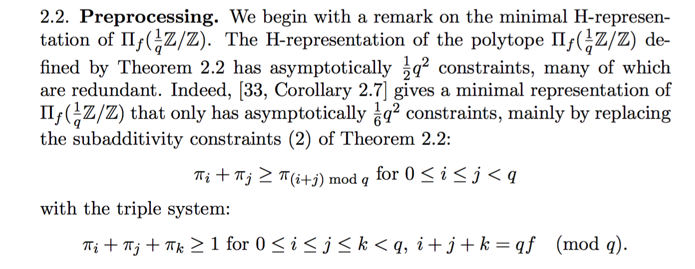
Case study: From the theory of subadditive functions
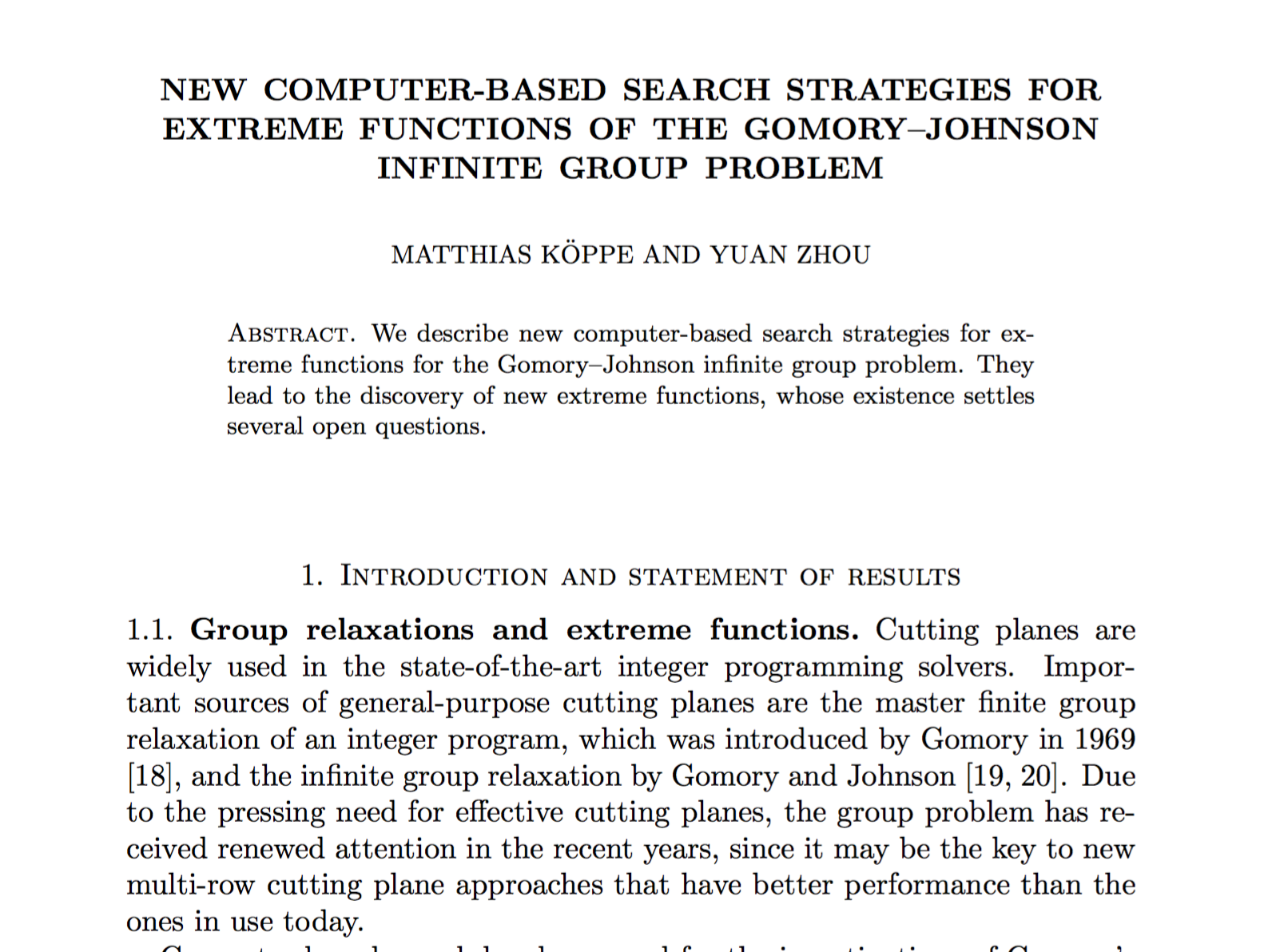
A family of polytopes with sparse inequalities, coefficients 1 and 2.
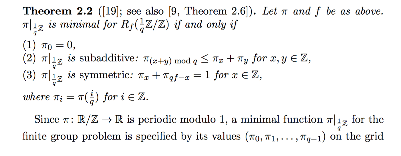
Wish to compute (and classify…) vertices
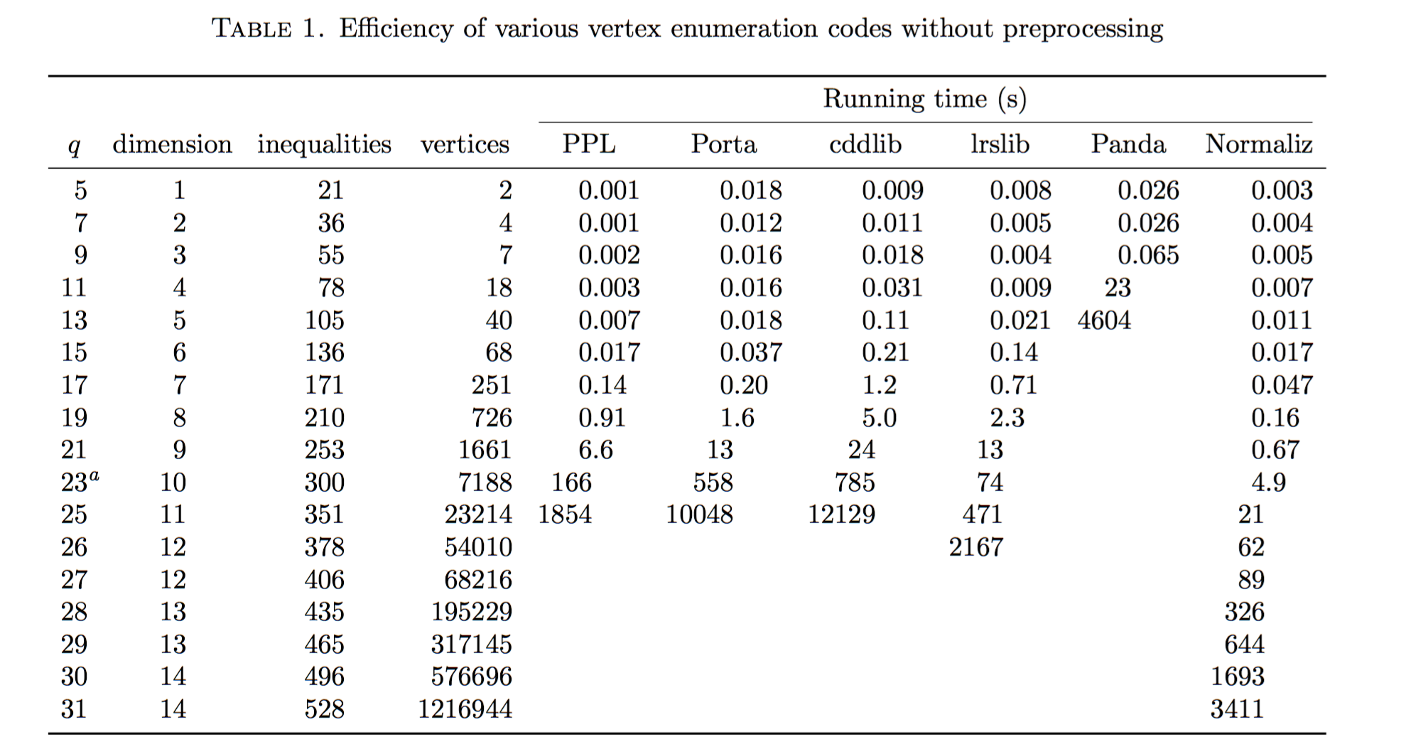
Could the problem be redundancy?
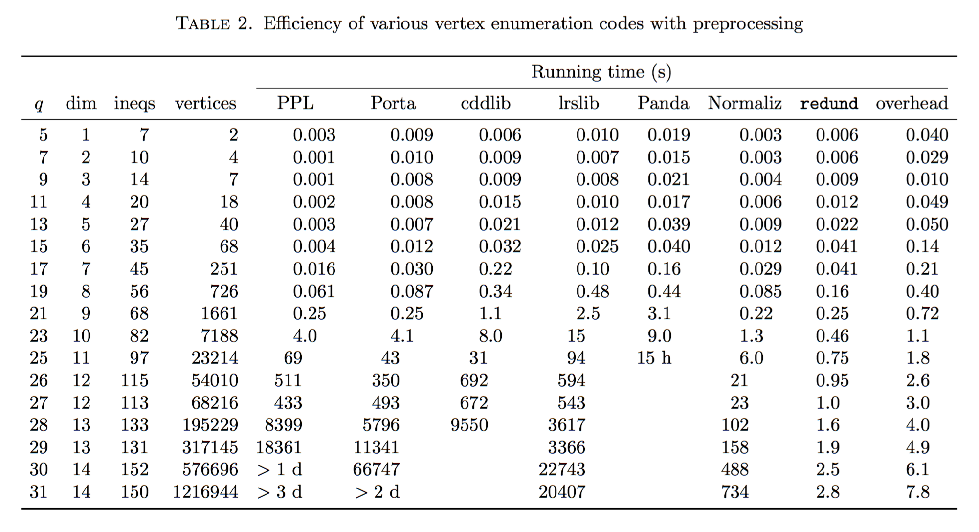
Why is it so fast?
| [BI] | W. Bruns and B. Ichim, Normaliz: algorithms for rational cones and affine monoids, J. Algebra 324 (2010), 1098–1113, https://doi.org/10.1016/j.jalgebra.2010.01.031. |
| [BIS] | W. Bruns, B. Ichim, and C. Söger, The power of pyramid decomposition in Normaliz, J. Symb. Comp. 74 (2016), 513–536, https://doi.org/10.1016/j.jsc.2015.09.003. |
The normaliz backend
Optional SageMath packages:
normaliz (Bruns et al.)
Provides file-based command-line interface (not used in Sage) and a C++ API
PyNormaliz (Gutsche)
Install:
./sage -i pynormaliz
Python code: sage.geometry.polyhedron.backend_normaliz (Köppe)
sage: P1_normaliz = Polyhedron(vertices = [[1, 0], [0, 1]], rays = [[1, 1]], backend='normaliz')  # optional - pynormaliz
sage: type(P1_normaliz)                                                                           # optional - pynormaliz
<class 'sage.geometry.polyhedron.parent.Polyhedra_ZZ_normaliz_with_category.element_class'>
sage: P2_normaliz = Polyhedron(vertices = [[1/2, 0, 0], [0, 1/2, 0]],                             # optional - pynormaliz
....:                 rays = [[1, 1, 0]],
....:                 lines = [[0, 0, 1]], backend='normaliz')
sage: type(P2_normaliz)                                                                           # optional - pynormaliz
<class 'sage.geometry.polyhedron.parent.Polyhedra_QQ_normaliz_with_category.element_class'>
The backend normaliz provides other methods such as
integral_hull, which also works on unbounded polyhedra.
sage: P6 = Polyhedron(vertices = [[0, 0], [3/2, 0], [3/2, 3/2], [0, 3]], backend='normaliz')  # optional - pynormaliz
sage: IH = P6.integral_hull(); IH                                                             # optional - pynormaliz
A 2-dimensional polyhedron in QQ^2 defined as the convex hull of 4 vertices
sage: P1_normaliz.integral_hull()                                                             # optional - pynormaliz
A 2-dimensional polyhedron in ZZ^2 defined as the convex hull of 2 vertices and 1 ray
TODO: trac ticket #25091 - Make further computation goals of Normaliz available as methods.
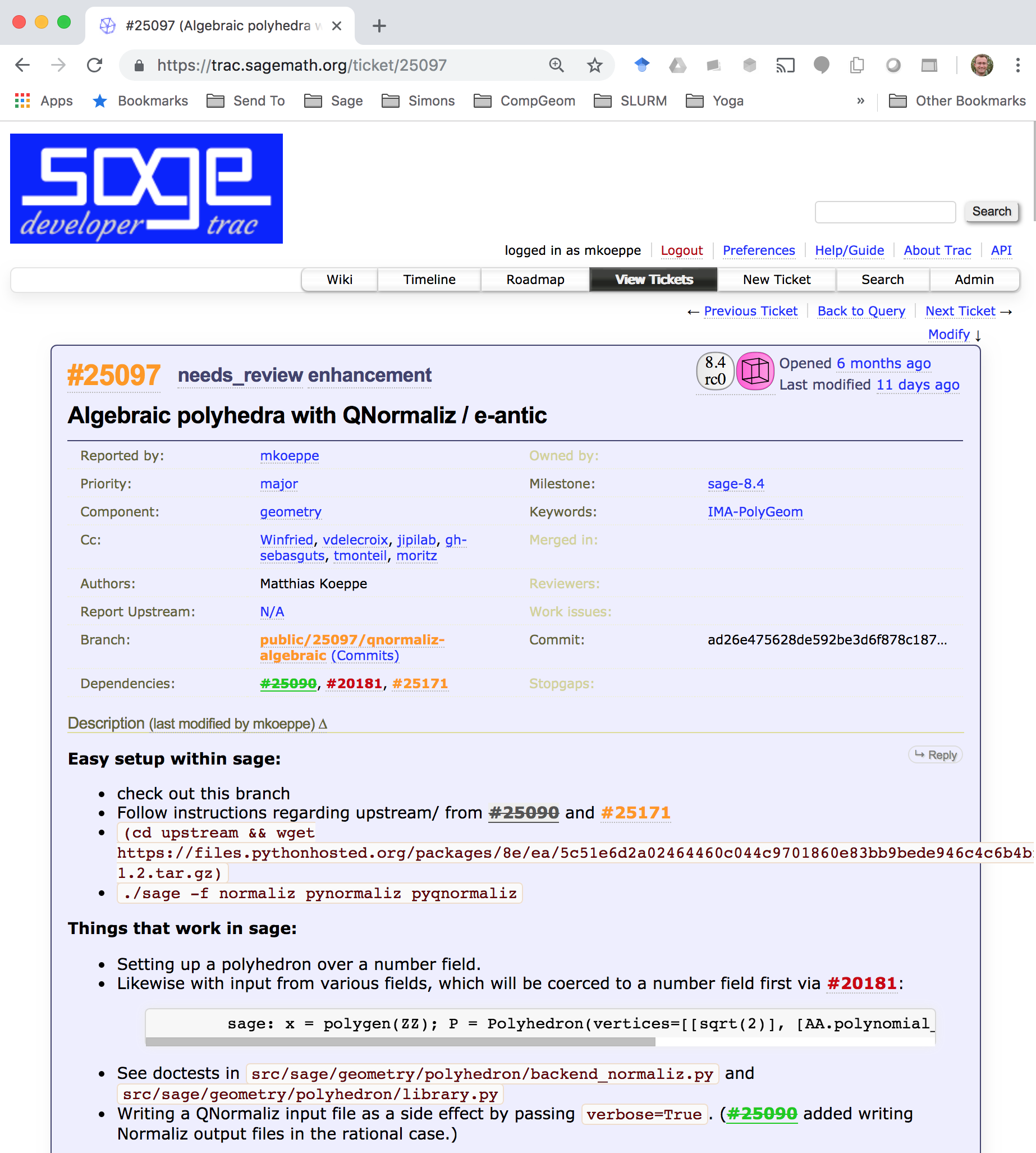
New: Polyhedra over algebraic number fields using QNormaliz
Our approach
(W. Bruns, V. Delecroix, S. Gutsche, M. Köppe, JP Labbe)
Take one of the best, actively developed and maintained polyhedral computation codes:
- Normaliz (Bruns et al.)
Suppress impulses such as:
- Fork the code
- “Because Python is such a clean language, we can just rewrite the whole thing in Python”
Instead: Convince upstream developer (Bruns) to generalize the code (without runtime cost; without source duplication (WIP)):
- QNormaliz (Bruns 2017-) - by using C++ templates, make parts of Normaliz code generic. Use a mock field (mpq_class) for prototyping
Prototype lower-level library for embedded number fields
- e-antic (Delecroix, 2016-),
building on state of the art libraries:
- arb (Johansson et al., 2013-),
- FLINT/ANTIC (Hart et al., 2013-).
Sage interfacing
- PyQNormaliz (Gutsche 2018),
- extended Sage backend_normaliz (Köppe 2018).
Status
Normaliz has QNormaliz/e-antic - stable release 3.6.3
Typical input file, normaliz/Qexample/dodecahedron-v.in:
amb_space 3
number_field min_poly (a^2 - 5) embedding [2.236067977499789 +/- 8.06e-16]
subspace 0
vertices 20
(-a + 3) (-a + 3) (-a + 3) 1
(2*a - 4) 0 (a - 1) 1
(-a + 3) (a - 3) (-a + 3) 1
(a - 1) (2*a - 4) 0 1
(a - 1) (-2*a + 4) 0 1
0 (a - 1) (2*a - 4) 1
0 (-a + 1) (2*a - 4) 1
(-2*a + 4) 0 (a - 1) 1
(a - 3) (-a + 3) (-a + 3) 1
(a - 3) (a - 3) (-a + 3) 1
(-a + 3) (-a + 3) (a - 3) 1
0 (a - 1) (-2*a + 4) 1
(-a + 3) (a - 3) (a - 3) 1
0 (-a + 1) (-2*a + 4) 1
(2*a - 4) 0 (-a + 1) 1
(-a + 1) (2*a - 4) 0 1
(-a + 1) (-2*a + 4) 0 1
(a - 3) (-a + 3) (a - 3) 1
(a - 3) (a - 3) (a - 3) 1
(-2*a + 4) 0 (-a + 1) 1
cone 0
Volume
Deg1Elements
IntegerHull
Sage interfacing: WIP at trac ticket #25097
We need your algebraic polytopes
Thank you!