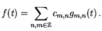
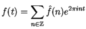
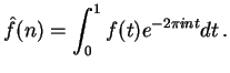
Motivated by the study of heat diffusion, Fourier asserted
that an arbitrary function ![]() in
in ![]() could be represented by a
trigonometric series
could be represented by a
trigonometric series
 |
 |
A good part of mathematical analysis developed since then
was devoted to the attempt to make Fourier's statement precise. Despite the
delicate problems of convergence, Fourier series are a powerful and
widely used tool in mathematics,
engineering, physics, and other areas. The existence of the Fast Fourier
Transform has extended this use enormously
in the past thirty years. Fourier expansions are not only
useful to study single functions or function spaces, they can also
be applied to study operators between function spaces. It is a well-known
fact that the trigonometric basis
![]() diagonalizes translation invariant operators on the interval
diagonalizes translation invariant operators on the interval ![]() ,
identified with the torus.
,
identified with the torus.
However the Fourier system is not adapted to represent local
information in time of a function or an operator, since the representation
functions themselves are not at all localized in time, we have
![]() for all
for all ![]() and
and ![]() . A local perturbation
of
. A local perturbation
of ![]() may result in a perturbation of all expansion
coefficients
may result in a perturbation of all expansion
coefficients
![]() . Roughly speaking the same
remarks apply to the Fourier transform.
The Fourier transform is an ideal tool to study stationary signals
and processes (where the properties are statistically invariant
over time). However many physical processes and signals are nonstationary,
they evolve with time, such as speech or music.
. Roughly speaking the same
remarks apply to the Fourier transform.
The Fourier transform is an ideal tool to study stationary signals
and processes (where the properties are statistically invariant
over time). However many physical processes and signals are nonstationary,
they evolve with time, such as speech or music.
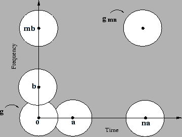
Let us take for instance a short segment of Mozart's Magic Flute (say thirty seconds and the corresponding number of samples, as they are stored on a CD). If we represent this piece of music as a function of time, we may be able to perceive the transition from one note to the next, but we get little insight about which notes are in play. On the other hand the Fourier representation may give us a clear indication about the prevailing notes in terms of the corresponding frequencies, but information about the moment of emission and duration of the notes is masked in the phases. Although both representations are mathematically correct, but one does not have to be a member of the Vienna Philharmonic Orchestra to find neither of them very satisfying. According to our hearing sensations we would intuitively prefer a representation which is local both in time and frequency, like music notation, which tells the musician which note to play at a given moment. Additionally such a local time-frequency representation should be discrete, so that it is better adapted to applications.
Dennis Gabor had similar considerations in mind, when he
introduced in 1946 in his ``Theory of Communication'' a method to represent
a one-dimensional signal in two dimensions, with
time and frequency as coordinates [Gab46].
Gabor's research in communication theory was driven by the question
how to represent locally as good as possible by a finite number of data
the information of a signal which is given a priori through
uncountably many function values ![]() . He was
strongly influenced by developments in quantum mechanics, in particular
by Heisenberg's uncertainty principle and by
the fundamental results of Nyquist and Hartley.
on the limits for the transmission of information over a channel.
. He was
strongly influenced by developments in quantum mechanics, in particular
by Heisenberg's uncertainty principle and by
the fundamental results of Nyquist and Hartley.
on the limits for the transmission of information over a channel.
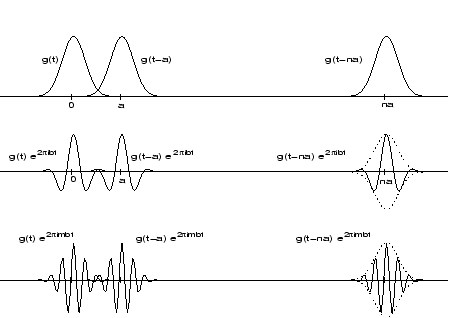
Gabor proposed to expand a function ![]() into a series of elementary functions,
which are constructed from a single building block by
translation and modulation (i.e. translation in the frequency domain).
More precisely he suggested to represent
into a series of elementary functions,
which are constructed from a single building block by
translation and modulation (i.e. translation in the frequency domain).
More precisely he suggested to represent ![]() by the series
by the series
 |
We could also say that the ![]() in (0.2)
are obtained by shifting
in (0.2)
are obtained by shifting ![]() along a lattice
along a lattice
![]() in the time-frequency plane.
If
in the time-frequency plane.
If ![]() and its Fourier transform
and its Fourier transform ![]() are essentially localized at
the origin, then
are essentially localized at
the origin, then ![]() is essentially localized at
is essentially localized at ![]() in the
time-frequency plane. Hence each such
elementary function
in the
time-frequency plane. Hence each such
elementary function ![]() essentially occupies a certain area (``logon'')
in the time-frequency plane. Each of the
expansion coefficients
essentially occupies a certain area (``logon'')
in the time-frequency plane. Each of the
expansion coefficients ![]() , associated to a certain area of the
time-frequency plane via
, associated to a certain area of the
time-frequency plane via ![]() , represents one quantum of information.
For properly chosen shift parameters
, represents one quantum of information.
For properly chosen shift parameters ![]() the
the ![]() cover the
time-frequency plane, as demonstrated in Figure 2.
cover the
time-frequency plane, as demonstrated in Figure 2.
 |
Gabor proposed to use the Gauss function and its translations and
modulations with shift parameters ![]() as elementary signals,
since they ``assure the best utilization of the information
area in the sense that they possess the smallest product of effective
duration by effective width'' [Gab46]. Recall that the
uncertainty principle inequality states that for all functions
as elementary signals,
since they ``assure the best utilization of the information
area in the sense that they possess the smallest product of effective
duration by effective width'' [Gab46]. Recall that the
uncertainty principle inequality states that for all functions
![]() and for all points
and for all points
![]() in the
time-frequency plane
in the
time-frequency plane
It is obvious that time series and Fourier series are limiting cases
of Gabor's series expansion.
The first one may be obtained by letting
![]() in (0.3),
in which case the
in (0.3),
in which case the ![]() approximate the delta distribution
approximate the delta distribution ![]() , in the
second case, the
, in the
second case, the ![]() become ordinary sine and cosine waves for
become ordinary sine and cosine waves for
![]() .
.
The idea to represent a function ![]() in terms of the time-frequency
shifts of a single atom
in terms of the time-frequency
shifts of a single atom ![]() did not only originate in communication
theory but somewhat 15 years earlier also in quantum mechanics. In an
attempt to expand general
functions (quantum mechanical states) with respect to states with minimal
uncertainty, John von Neumann [vN55] introduced
in 1932 a set of coherent states on a lattice with lattice
constants
did not only originate in communication
theory but somewhat 15 years earlier also in quantum mechanics. In an
attempt to expand general
functions (quantum mechanical states) with respect to states with minimal
uncertainty, John von Neumann [vN55] introduced
in 1932 a set of coherent states on a lattice with lattice
constants ![]() in the phase space with position
and momentum as coordinates (here
in the phase space with position
and momentum as coordinates (here ![]() is the
Planck constant).
These states, associated with the Weyl-Heisenberg group
are in principle the same used by Gabor.
Therefore the system
is the
Planck constant).
These states, associated with the Weyl-Heisenberg group
are in principle the same used by Gabor.
Therefore the system
![]() is also called Weyl-Heisenberg system,
and the time-frequency lattice with
lattice constants
is also called Weyl-Heisenberg system,
and the time-frequency lattice with
lattice constants ![]() is also referred
to as von Neumann lattice.
We recommend the book of Klauder and Skagerstam for an excellent
review on coherent states [KS85].
is also referred
to as von Neumann lattice.
We recommend the book of Klauder and Skagerstam for an excellent
review on coherent states [KS85].
Only two years after Gabor's paper, Shannon published ``A Mathematical Theory of Communication'' [Sha48]. It should be emphasized that the temporal coincidence is not the only connection between Gabor theory and Shannon's principles of information theory. Both, Shannon and Gabor, tried to ``cover'' the time-frequency plane with a set of functions, transmission signals for digital communication in Shannon's case and building blocks for natural signals in Gabor's case. While Gabor explicitly suggested the Gaussian function and Weyl-Heisenberg structure, Shannon only emphasized the relevance of orthonormal bases without explicitly suggesting a signal set design. Yet, the determination of a critical density (referred to as degrees of freedom per time and bandwidth in Shannon's work) was one of the key mathematical prerequisites for Shannon's famous Capacity Theorem. In summary, both Gabor and Shannon worked about the same time on communication engineering problems related to Heisenberg uncertainty and phase space density, where at that time only very few mathematicians, most prominently von Neumann, had touched upon their basics. Note, however, that Shannon's work certainly had a greater impact on the engineering community than the work of Gabor.
Two questions arise immediately with an expansion of the form (0.6):
While Gabor was awarded the Nobel Prize in Physics in 1971 for the conception of holography, his paper on ``Theory of Communication'' went almost unnoticed until the early 80's, when the work of Bastiaans and Janssen refreshed the interest of mathematicians and engineers in Gabor analysis. The connection to wavelet theory1 and the increasing interest of scientists in signal analysis and frame theory was then very much influenced by the work of I. Daubechies. But before we proceed to the 80's let us go back to the 30's and 40's and follow the development of Gabor theory from the signal analysis point of view.