Naoki's Selected Scientific Contributions

Autocorrelation Wavelets
In June 1990, I attended the legendary "Ten Lectures on Wavelets" delivered by Ingrid Daubechies, held at Univ. of Lowell, MA. After learning various properties of Daubechies wavelets, I wanted to construct a shift-invariant multiresolution representation of an input signal for the purpose of signal analysis and interpretation. The geometric property of the Daubechies wavelets, i.e., lack of symmetry and fractal-like shapes, were not suitable for that purpose. Then, I observed that the autocorrelation functions of the father wavelets of Daubechies's coincide with the so-called fundamental functions of the symmetric iterative interpolation scheme proposed by Deslauriers and Dubuc in 1989. This led to the autocorrelation shell signal representation developed in collaboration with Gregory Belkin.
Let $\Phi(x)$ and $\Phi(x)$ be the autocorrelation functions of Daubechies father and mother wavelet functions $\phi(x)$ and $\psi(x)$ corresponding to the quadrature mirror filter with $L$ taps, respectively, i.e., $$\Phi(x) := \int_{-\infty}^{+\infty} \phi(y) \phi(y-x) \mathrm{d}y, \quad \Psi(x) := \int_{-\infty}^{+\infty} \psi(y) \psi(y-x) \mathrm{d}y.$$

Fathers with $L=4$: (a) $\Phi(x)$; (b) $\phi(x)$; (c) $\hat{\Phi}(\xi)$; (d) $\hat{\phi}(\xi)$.

These functions have several remarkable properties:

Both $\Phi$ and $\Psi$ are symmetric;
$\Phi$ is a fundamental function for iterative interpolation, i.e., $\Phi(0) = 1$ while $\Phi(n) = 0, \forall n \in \mathbb{Z}\!\setminus\!\!\!\{0\}$; $L=2$ corresponds to the piecewise linear interpolation while $L \to \infty$ corresponds to the bandlimited interpolation;
$\Psi$ has vanishing moments of order from 0 to $L-1$ while $\Phi$ has those of order from 1 to $L-1$ while $\psi$ has those of order from 0 to $L/2$ and $\phi$ does not have vanishing moment property (unless using more special ones like coiflets;
$\Psi(x) = 2\Phi(2x) - \Phi(x)$, which is like the Difference of Gaussians (DoG) filter;
$\hat{\Psi}(\xi) = O(\xi^L)$ when $\xi \approx 0$, i.e., convolving an input signal with $\Psi(x)$ essentially behaves as applying pseudo-differential operator to that signal.

Unlike wavelet-based orthonormal representations, this representation has: 1) symmetric analyzing functions; 2) shift invariance; 3) associated iterative interpolation schemes; and 4) a simple algorithm for finding the locations of the multiscale edges as zero crossings. We also developed a non-iterative method for reconstructing signals from their zero crossings (and slopes at these zero crossings) in our representation. We were influenced by the famous conjecture by David Marr: an input image can be determined by its multiscale edge information (i.e., locations and strengths of such edges), and its refined version proposed by Stephane Mallat using wavelet maxima. Yves Meyer found counterexamples to these conjectures in early 1990s. Our method reduces the reconstruction problem to that of solving a system of linear algebraic equations, and makes everything quite explicit.
I first reported our results briefly at the IEEE ICASSP in San Francisco in March 1992, and a bit more detail at the "Wavelet and Applications" International Conference, the first of its kind, held in Toulouse, France in June 1992. The latter conference, organized by Sylvie Roques, was really memorable: I met all the important players in this field including Yves Meyer and David Donoho , to whom I handed my technical report on this subject. The official journal version appeared in the special issue on wavelets of the IEEE Transactions on Signal Processing in Dec. 1993. See also my talk slides as well as a more complete technical report that contains more information than the published journal version.
The autocorrelation wavelets has been studied and applied further for various time series data, etc.; see, e.g., the work of Guy Nason and his collaborators. Also, David Donoho 's "interpolating wavelet transform" is closely related to our autocorrelation wavelets.

Simultaneous Noise Suppression and Signal Compression using Basis Dictionaries and the Minimum Description Length Criterion
After reading an inspiring paper on image partitioning by Yvan Leclerc followed by taking a graduate course on information theory at Yale offered by Andrew Barron, I got interested in the concept of the Minimum Description Length (MDL) originally introduced by Jorma Rissanen. My interest in MDL was further cemented after I took a tutorial titled "MDL Methods in Image Analysis and Computer Vision," delivered by Wayne Niblack (IBM Research) at the CVPR conference held in June 1993 in NYC. To simultaneously denoise and compress a given noisy signal effectively, it is important to realize that a signal component in the noisy data may be represented efficiently by one or more of the bases in the basis library whereas the noise component cannot be represented efficiently by any basis in the library. I thought that the MDL criterion should be a fantastic criterion to select:

a basis among several different best bases each of which was selected from different basis dictionaries such as the Haar- Walsh wavelet packet dictionary, a more general Daubechies wavelet packet dictionary, and local cosine dictionary, etc.; and
significant coefficients to keep relative to a given basis.

The idea of choosing a best basis from a basis dictionary was proposed in the groundbreaking paper by Raphy Coifman and Victor Wickerhauser. Even if we can select the best of the best bases for a given input signal from a collection of the best bases selected from a set of basis dictionaries, we always face the problem: how many coefficients should we keep (or equivalently, how can we determine the cutoff threshold)? The MDL criterion gives the best compromise between the fidelity of the estimation result to the data (noise suppression) and the efficiency of the representation of the estimated signal (signal compression): it selects the best of the best bases and the best number of terms to be retained out of various bases in the library in an objective manner. Because of the use of the MDL criterion, my algorithm is free from any parameter setting or subjective judgments (except that the selection of the basis dictionaries to be considered).

Denoising/compression of a natural radioactivity profile
of subsurface formation:
(a) Original signal with 1024 samples;
(b) Estimation using the top 77 best-basis coefficients;
(c) Residual error between (a) and (b).

I initially made a presentation on this idea at the SPIE Conference on Wavelet Applications held in April 1994 in Orlando, FL. In that conference, I met Efi Foufoula-Georgiou who asked me to submit a full version of my paper to "Wavelets in Geophysics", the book she was editing, which was eventually published from Academic Press in 1994. This paper also served as an introduction to or a tutorial on the MDL principle, and is still getting many citations. David Donoho and Iain Johnstone also cited my paper in their paper on ideal denoising via an ONB chosen from a library of bases.

Local Discriminant Basis
By Summer of 1992, Victor Wickerhauser generalized the original best-basis algorithm—which was designed for a single input signal—for a collection of signals, which he called the joint best basis (JBB). This can be viewed as a time-frequency localized version of the Principal Component Analysis (PCA) or the so-called Karhunen-Loève Basis (KLB). PCA and JBB should be used for a single class of signals that share the same important features, and do not work for signal classification in general. Some critical features that differentiates different signal classes may be buried in the small PCA/JBB coordinates. What was really needed was to develop a time-frequency localized version of Linear Discriminant Analysis (LDA). In November 1993, while I was working at home (then in Brookfield, CT) and viewing beautiful foliage from the window, I suddenly hit upon a good idea: replacing the original minimum entropy cost function used in the JBB by the Kullback-Leibler divergence (a.k.a. relative entropy) between time-frequency energy distributions of signal classes. More precisely, this method first decomposes available training signals in a time-frequency dictionary, which is a large collection of basis functions (e.g., wavelet packets and local trigonometric functions) localized both in time and in frequency. Then, signal energies at the basis coordinates are accumulated for each signal class separately to form a time-frequency energy distribution per class. Based on the differences among these energy distributions (measured by a certain "distance" functional, e.g., the Kullback-Leibler divergence, the Hellinger distance, etc.), a complete orthonormal basis called LDB, which can see the distinguishing signal features among signal classes, is selected from the dictionary. After the LDB is determined, the expansion coefficients in the most important several coordinates (features) are fed into any standard classifier such as LDA or classification tree (CT). Finally, the corresponding coefficients of test signals are computed and fed to the classifier to predict their class labels. The computational cost to select the LDB for a given set of training signals, say, totally $m$ signals each of which has $n$ samples, is is relatively low: $O(m n [\log n]^p)$, where $p=1$ for a wavelet packet dictionary while $p=2$ for a local trigonometric dictionary.
The following example, "signal shape classification," which has become popular among many researchers, illustrates the point of LDB. My original motivation was to classify geophysical well logs into different sedimentary facies classes. In this example, we try to classify synthetic noisy signals with various shapes, amplitudes, lengths, and positions into three possible classes. More precisely, sample signals of the three classes were generated by: $$ \begin{aligned} c(i) &= (6 + \eta) \cdot \chi_{[a,b]}(i) + \epsilon(i) \\ b(i) &= (6 + \eta) \cdot \chi_{[a,b]}(i) \cdot (i-a)/(b-a) + \epsilon(i) \\ f(i) &= (6 + \eta) \cdot \chi_{[a,b]}(i) \cdot (b-i)/(b-a) + \epsilon(i) \end{aligned} \quad \begin{aligned} &\text{for }\unicode{x201C}\text{cylinder}\unicode{x201D}\text{ class,}\\ &\text{for }\unicode{x201C}\text{bell}\unicode{x201D}\text{ class,}\\ &\text{for }\unicode{x201C}\text{funnel}\unicode{x201D}\text{ class,} \end{aligned} $$ where $i=1,\ldots,128$, $a$ is an integer-valued uniform random variable on the interval $[16,32]$, $b-a$ also obeys an integer-valued uniform distribution on $[32,96]$, $\eta$ and $\epsilon(i)$ are the standard normal variates, and $\chi_{[a,b]}(i)$ is the characteristic (or indicator) function on the interval $[a,b]$. The following figure shows five sample waveforms from each class. If there is no noise, we can characterize the "cylinder" signals by two step edges and constant values around the center, the "bell" signals by one ramp and one step edge in this order and positive slopes around the center, and the "funnel" signals by one step edge and one ramp in this order and negative slopes around the center.

Sample signal shape classification waveforms:
(a) "cylinder"; (b) "bell"; (c) "funnel".

For each class, I generated 100 training signals and 1000 test signals. The 12-tap coiflet filter was used for the LDB selection shown above. Then the 10 most important coordinates were selected. Only the top two vectors were used for classification in LDA case because this is a three-class classification problem. These LDA vectors are very noisy and it is difficult to interpret what information they captured. On the other hand, we can observe that the top 10 LDB vectors are located around the edges or the centers of the signals. Also note that some of the vectors work as a smoother (low pass filter) and the others work as a edge detector (band pass filter), so that the resulting expansion coefficients carry the information on the edge positions and types. The misclassification rates (averages over 10 simulations) in this case are:

Method	Training (%)	Test (%)
LDA on raw inputs	0.83	12.31
CT on raw inputs	2.83	11.28
LDA on top 10 LDB coordinates	7.00	8.37
CT on top 10 LDB coordinates	2.67	5.54
CT on all LDB coordinates	2.33	7.60

As expected, LDA applied to the original coordinate system was almost perfect with respect to the training data, but it adapted too much to the features specific to the training data, and lost its generalization power; when applied to the new test dataset, it did not work well. The best result was obtained using the CT on the top 10 LDB coordinates in this example. The misclassification rates of the training data and the test data are very close here; that is, the algorithm really "learned" the structures of signals. This best CT is shown in the above figure. If the tree-based classification is combined with the coordinate system capturing local information in the time-frequency plane, the interpretation of the result becomes so explicit and easy: in the above CT figure, we find that the LDB coordinate #1 is checked first. If this is less than 10.0275, it is immediately classified as "bell." From the middle figure (b), we observe that the LDB function #1 is located around $i=30$ which, in fact, coincides with the starting position (the parameter $a$ in the formulas) of various signals. Around this region, both the cylinder and the funnel signals have sharp step edges. On the other hand, the bell signals start off linearly. Thus CART algorithm found that the LDB function #1 is the most important coordinate in this example. The separating the cylinder class from the funnel class turned out to be more difficult because of the large variability of the ending positions. This resulted in the more complicated structure of the right branch from the root node. But we can still obtain the intuitive interpretation: the first node in the right branch (with "cylinder" label) from the root node is split into either "funnel" or "cylinder" depending on the LDB coordinate #5 which is located around the middle of the axis ($i=64$). If there were no noise, the cylinder signals would have constant values around this area whereas the funnel signals would decrease linearly here; the LDB obtained this important information by removing the noise. One can continue the interpretation in a similar manner for all remaining nodes.
I initially wrote an extended summary about the LDB (as well as Local Regression Basis (LRB) with my PhD adviser, Raphy Coifman, and published it in Comptes Rendus de l'Acadéemie des Sciences, Série I. Then, I presented a bit more details on the LDB part at the SPIE Conference on Wavelet Applications in Signal and Image Processing II held in San Diego, CA, in July 1994, where I got the Best Paper Award. Because of this, we were invited to submit our longer journal version of the paper to the special issue of the Journal of Mathematical Imaging and Vision, which appeared in Dec. 1995. Also, in May 1995, I was invited to give a talk about the LDB at the Joint Yale-KTH Royal Institute of Technology in Stockholm, Sweden. Lennart Carleson was in the audience, and he suggested that I should apply the LDB algorithm for classifying birds songs, which consists of various chirps. He was right in the sense that the wavelet packets and local cosines used in the LDB algorithm have higher spectral resolution than the conventional wavelets. As of today, however, I haven't really tacked this problem yet. Later on in 2017, my PhD student, Alex Berrian and I realized that better tools are required for bioacoustic signal analysis than the wavelet packets and local cosines, and we developed the quilted short-time (or windowed) Fourier transform equipped with "chirped" windows to handle rapidly-changing nonstationary chirp signals, which I plan to describe later in this page.
Over the years, the LDB algorithm has become popular: it has been applied to a variety of classification problems including geophysical acoustic waveform classification, radar signal classification, and classification of neuron firing patterns of monkeys to different stimuli, etc.

Despite its popularity and effectiveness, by early 1996, I realized that the difference between time-frequency energy distributions among signal classes is not always the best one to use for classification and discrimination tasks: such energy distributions are blind to differences in sign and phase information of the expansion coefficients. To eliminate such problems, together with Raphy Coifman and his associates, Frank Geshwind and Fred Warner, I proposed to use the empirical probability density functions (pdfs) of each coordinate over different classes in a given basis dictionary. Any kernel density estimation methods can be used for empirical pdf estimation, but we really liked a simpler yet efficient Averaged Shifted Histogram (ASH). This leads to the use of true Kullback-Leibler divergence between pdfs in the LDB algorithm instead of the coordinatewise time-frequency energy distributions. The final version of our paper, although it took a longer time to finish than I had expected, it was published in the journal Pattern Recognition in Dec. 2002.

Around mid 2005, I learned the concept of Earth Mover's Distance (EMD), and felt that the EMD could be used as yet another cost functional to select an LDB. It took some time due to the other projects, but with the help of my PhD student, Brad Marchand, I developed and examined the performance of the new version of the LDB algorithm using the EMD. We demonstrated its capability of detecting features that can be missed using other versions of LDBs. Our EMD-based LDB can also be adapted to use new training data as it is provided. In comparison to the LDB using the ASH-type empirical pdf estimate, our new LDB algorithm has fewer parameters to tweak and avoids the difficult task of estimating reliable epdfs, which make this new algorithm more robust. We also demonstrated that the new LDB revealed better separation of classes with less training and less susceptible to outliers for certain classification problems, but as one can imagine, its performance depends on the problems at hand, i.e., for certain problems, the good old LDB using the time-frequency energy distributions performed best. We published our findings and results as a book chapter in the book "Multiscale Signal Analysis and Modeling" (X. Shen and A. I. Zayed, eds.), Springer, 2013, which was dedicated to Gilbert Walter on the occasion of his 80th birthday.

Local Regression Basis
Soon after I hit on the idea of the LDB, developed its computational algorithm, and conducted numerical experiments, I realized the necessity of using a different basis selection criterion for regression problems. For regression problems, I wanted to select a good set of coordinates in a given basis dictionary that offer good interpretability with small prediction error. This led to the idea of the Local Regression Basis, using the prediction error (e.g., the residual sum of squares, etc.) using a regression method of one's choice (e.g., linear regression or regression tree) at each subspace as the basis selection criterion in a basis dictionary. I need to note that this cost functional is non-additive unlike the discriminant measures used in the LDB algorithms since the prediction error using the coordinates in a union of two subspaces may be smaller than the prediction error in each of these two subspaces.
My initial idea was published as one section in the extended summary paper mentioned in the LDB section, which appeared in Comptes Rendus de l'Acadéemie des Sciences, Série I, in July 1994. But I wrote a full-length journal version of the LRB with geophysical applications, i.e., estimation of volume fraction of minerals in geological formations using the acoustic waveforms propagated those formations in the journal Geophysics, which appeared in late 1997.

Least Statistically-Dependent Basis
In summer of 1997, I moved from industry (Schlumberger) to academia (UC Davis). Around that time, I got interested in the concept of statistical independence of a given set of coordinates: if we could truly find such a set of coordinates, we could simulate a high-dimensional stochastic process by sampling each coordinate separately (i.e., a product of 1D stochastic simulations). There was already a method called Independent Component Analysis (ICA), which had drawn attention of signal processors and statisticians. Of course, for given realizations of a stochastic process, ICA may not be able to find a truly statistically independent set of coordinates or components in general because ICA merely finds an optimal solution for either minimization of mutual information or maximization of non-Gaussianity. However, the ICA algorithms influenced my thinking, and subsequently I reached the idea of Least Statistically-Dependent Basis (LSDB) selectable from a basis dictionary. The LSDB uses the minimization of the mutual information of the distributions of the basis coefficients as a measure of statistical dependence, which in turn is equivalent to minimization of the sum of the differential entropy of each coordinate in the basis dictionary. In this sense, the LSDB algorithm can be viewed as the best-basis version of the ICA. The key observations are:

Mutual information of a high-dimensional stochastic process $\boldsymbol{X} \in \mathbb{R}^d$ is merely the relative entropy between the original pdf and the product of its marginal pdf's, i.e., $$ I(\boldsymbol{X}) := \int f_{\boldsymbol{X}}(\boldsymbol{x}) \log \frac{f_{\boldsymbol{X}}(\boldsymbol{x})}{\prod_{i=1}^d f_{X_i}(x_i)} \mathrm{d}\boldsymbol{x} = -H(\boldsymbol{X}) + \sum_{i=1}^d H(X_i), $$ where $H(\boldsymbol{X})$ is differential entropy of $\boldsymbol{X}$, i.e., $\displaystyle H(\boldsymbol{X}) := -\int f_{\boldsymbol{X}}(\boldsymbol{x}) \log f_{\boldsymbol{X}}(\boldsymbol{x}) \mathrm{d}\boldsymbol{x}$.
Differential entropy of linearly-transformed process $\boldsymbol{Y}=A\boldsymbol{X}$ where $A \in \mathbb{R}^{d \times d}$ is simply: $$ H(\boldsymbol{Y})= H(A\boldsymbol{X}) = H(\boldsymbol{X})+\log |\det(A)|.$$
Hence, if $A$ is a volume-preserving transformation, i.e., if $A \in SL(d, \mathbb{R})$, the special linear group of degree $d$, then $ H(A\boldsymbol{X}) = H(\boldsymbol{X}) $.

Clearly, any orthonormal basis matrix $B \in O(d)$ belongs to $SL(d, \mathbb{R})$, hence, under the basis dictionary setting, the LSDB of a given set of realizations is simply the basis that minimizes the sum of the coordinatewise differential entropy, each of which can be estimated by any kernel density estimation methods or a simpler ASH. This criterion is different from that of the JBB briefly described above, which can be viewed as the best-basis version of the PCA/KLB. I demonstrated the usefulness of the LSDB for image approximation and modeling and compare its performance with that of PCA/KLB and JBB using a collection of real geophysical acoustic waveforms and an image database of human faces.

Since the number of training images is 72, the KLB approximation here is simply a projection of a target image onto the 72 dimensional subspace spanned by the 72 "eigenfaces" (the computable KLB vectors). This original face image in belongs to the test dataset, not to the training dataset. If the target image were in the training dataset, then the KLB approximation would be perfect. However, because the target image is not in the training dataset, the approximation using these 72 KLB vectors is not impressive. In fact, it is not clear whether one can judge whether this approximation represents the same person as the original image. Using this standard KLB, we cannot do better than this. This essentially implies that the faces in the "Rogues' Gallery" dataset do not obey the multivariate Gaussian distribution, and the mean and the covariance matrix computed from the training dataset did not capture the variability of the faces in the test dataset. Now, let us examine the JBB and LSDB approximations. Compared to the KLB, which has only 72 meaningful vectors in this case, we can compute a complete basis for both the JBB and the LSDB. Note that the LSDB nicely split the faces into a set of meaningful regions. In particular, the regions around the eyes are split into a set of small segments, and most of the background regions are split into a larger segments. It is interesting to note that Kirby and Sirovich carefully cropped the oval-shaped portion of the faces containing the eyes, noses, and mouths and removed all the background and most of the hair portion for their approximations since "it significantly reduced the accuracy of the expression." We note that this natural splitting was done automatically in our case. On the other hand, JBB simply splits the images into four quadrants. The 72 term approximations by the JBB and LSDB shown in the above figure are not necessarily better than the one by the KLB. However, they offer much more than the KLB. With the JBB and LSDB, we can use more terms to perform better approximation. With the most energetic 800 terms (i.e., about 6% of the total number of dimensions) instead of 72 terms, we can get the very good approximation as shown below.

In this figure, we compare the performance of the various adaptive and non-adaptive bases. As non-adaptive bases, we used the wavelet basis with the 12-tap coiflet filter and the fixed folding local cosine transform (FLCT) by splitting the images homogeneously into a set of subimages of $8 \times 8$ pixels. The latter is very close to the block Discrete Cosine Transform (DCT) algorithm used in the JPEG image compression standard, although the FLCT has less edge effect than the block DCT. As adaptive bases, we used the JBB with multiple folding local cosine transform (MFLCT), and the LSDB with MFLCT. We observe that the LSDB approximation perceptually performs best, especially around important signatures such as the eyes, nose, and mouth.
I first presented the idea of the LSDB at the SPIE Conference on Wavelet Applications in Signal and Image Processing VI, in San Diego, in July 1998 as well as the Asilomar Conference on Signal, Systems & Computers, in Oct. 1998. The final journal paper version appeared in the journal Pattern Recognition, in Sep. 2001.

Sparsity vs Statistical Independence This subject is of course quite related to the LSDB, and it started with my conversation with David Mumford in March 1997 whom I invited to Schlumberger for his colloquium talk. He suggested to me that I should contact Bruno Olshausen who then recently joined UC Davis who did a remarkable work with David Field about the emergence of receptive field profiles similar to Gabor functions, i.e., multiscale, oriented, localized, and bandpass functions, by seeking a basis that sparsifies a set of input natural image segments. They wanted to shed light on understanding response properties of visual neurons, e.g., retinal ganglion cells. Furthermore, David Donoho , inspired by Olshausen and Field, proposed the so-called Sparse Component Analysis using the $\ell^p$-norm with $ 0 < p \leq 1$ as a measure of sparsity, and conducted rigorous mathematical analysis on such empirical observations.
On the other hand, in 1980s (or even earlier) Satosi Watanabe and Horace Barlow independently proposed the minimum entropy coding instead of sparse coding. More precisely, Watanabe suggested that the whole pattern recognition effort can be viewed as "a quest for minimum entropy" while Barlow suggested the factorial coding to explain the role of the massive flow of sensory information entered to our brains. Also, the researchers working on ICA, e.g., Tony Bell and Terry Sejnowski, derived results similar to those of Olshausen-Field.
Hence, I naturally got very interested in understanding the subtle difference between the sparsity and the statistical independence. One can see the difference easily in the following simple example. Let us consider a simple process $\boldsymbol{X}=(X_1,X_2)$ where $X_1$ and $X_2$ are independently and identically distributed as the uniform distribution on $[-1,1]$. Then, let us consider all possible rotations around origin as a basis dictionary, i.e., $\mathcal{D}=O(2)$, all possible 2D rotations. Then, the sparsity and independence criteria select completely different bases as shown in the following figure. This example clearly demonstrates that the sparsest coordinates and the statistically independent coordinates are generally different.

I published at least three papers on this subject. My first paper was to examine the difference between sparsity and statistical independence using appropriate criteria for the best-basis selection algorithm. This was done jointly with my then PhD student, Brons Larson, and my intern from École Polytechnique, Bertrand Bénichou. In that paper, we used synthetic stochastic processes (e.g., spike, ramp, and generalized Gaussian processes) as well as the image patches of natural scenes. Our experiments and analysis suggested the following:

Both sparsity and statistical independence criteria selected similar bases for most of our examples with minor differences except the case of 2D uniform distributions shown above;
Sparsity is more computationally and conceptually feasible as a basis selection criterion than the statistical independence, particularly for data compression;
The sparsity criterion can and should be adapted to individual realization rather than for the whole collection of the realizations to achieve the maximum performance;
The importance of orientation selectivity of the local Fourier dictionary was not clearly demonstrated due to the boundary effect caused by the folding and local periodization.

These observations seem to encourage the pursuit of sparse representations rather than that of statistically independent representations. Also, I should mention that Item 4 above led to my project of polyharmonic local trigonometric transforms.

My second paper on this subject, co-authored with Bertrand Bénichou, analyzed a simple yet interesting stochastic process that we named as spike process in a more mathematically rigorous manner. The spike process puts a unit impulse at a random location in an $d$-dimensional vector for each realization. For this process, we obtained the following results:

The standard basis is the best in terms of sparsity for any $d \geq 2$ among $GL_a(d,\mathbb{R}) := a^{1/d}\cdot SL(d,\mathbb{R})$ where $a > 0$ is a given constant [which clearly includes $O(d)$];
The standard basis is again the best in terms of statistical independence among $O(d)$ for $d \geq 5$, but there exists another basis achieving the same optimality as the standard basis; for $2 \leq d \leq 4$, the standard basis is not the best orthonormal basis in terms of statistical independence;
The best basis in statistical independence among $GL(d,\mathbb{R})$ with $d \geq 2$, is not the standard basis;
The best basis in statistical independence is not unique in general, and there even exist those which make the inputs completely dense;
There is no linear invertible transformation that achieves the true statistical independence for $d > 2$.

This was initially presented as an invited lecture as a part of the NSF-CBMS Regional Research Conference on "Interactions of Harmonic Analysis, Statistical Estimation, and Data Compression" whose main lecturer was David Donoho , which was held in May 2000 at University of Missouri-St. Louis. Many of the lectures in this conference was published in a book titled "Beyond Wavelets" edited by Grant Welland.

My third paper analyzed an extension of the spike process called the generalized spike process: putting a single spike with amplitude sampled from the standard normal distribution at a random location in an otherwise zero vector of length $d$. I proved that both the Best Sparsifying Basis (BSB; measured by the $\ell^p$-norm with $0 < p \leq 1$) and the Kurtosis Maximizing Basis (KMB) select the standard basis, if the basis search is restricted within $O(d)$. If basis search is extended to $SL(d,\mathbb{R})$, then I proved the BSB exists and is again the standard basis, whereas the KMB does not exist. Thus, the KMB is rather sensitive to the orthonormality of the transformations, while the BSB seems insensitive. These results provide new additional support for the preference of the BSB over the LSDB/KMB for data compression. This paper also included my explicit computation of the BSB for Yves Meyer's discretized ramp process. I should note that KMB is very closely related to the LSDB discussed above: the marginal differential entropy of the $i$th coordinate of a basis, say, $H(Y_i)$, is approximated by $$ H(Y_i) = -\frac{1}{48}\kappa(Y_i) = -\frac{1}{48}(\mu_4(Y_i)-3\mu_2^2(Y_i)),$$ where $\mu_k(Y_i)$ is the $k$th central moment of $Y_i$, and $\kappa(Y_i)/\mu_2^2(Y_i)$ is called the kurtosis of $Y_i$. The above formula was derived by Pierre Comon in his famous paper using the Edgeworth expansion. Here, I used the unnormalized version, i.e., $\kappa(Y_i)$. Hence, minimizing the sum of the marginal differential entropy in the LSDB corresponds to maximizing the sum of the (unnormalized) kurtosis in the KMB.
Dennis Healy and Dan Rockmore invited me to give a seminar at the Summer Graduate Program in Modern Signal Processing, which they ran at the Mathematical Sciences Research Institute in Berkeley, CA, in June 2001. This resulted in a book chapter in the book "Modern Signal Processing," which Dennis and Dan edited.

Polyharmonic Local Trigonometric Transforms I had been frustrated by the boundary/edge effect of the Fourier series and transform for a long time. For example, let us consider a very smooth function, say $f \in C^\infty[0,1]$ supported on the unit interval $[0,1]$, but not periodic with period 1. Then, its Fourier coefficients $\hat{f}(k)$ decays slowly, i.e., $O(1/k)$ as $k \to \pm\infty$, and creates the well-known Gibbs phenomenon. This is because the periodic extension of such $f$ becomes a discontinuous function due to the mismatch at the head and the tail in general: $f(0) \neq f(1)$ even if the original $f$ supported on $[0,1]$ has $C^\infty$ smoothness! This would become a serious issue particularly when we consider a localized version of the Fourier series/transform. In order to avoid this, the use of the short-time (or windowed) Fourier transform (STFT) has become quite popular in many fields. This is because multiplying a good window function around a local segment of an input signal makes that segment approximately a smooth periodic function. The discretized version of the STFT under certain conditions forms a frame and hence is invertible, but it does not provide a convenient dictionary of orthonormal bases. This led to the development of local cosine transforms of Coifman and Meyer, and lapped orthogonal transform of Henrique Malvar.
Along this direction, my PhD student, Brons Larson and I proposed the continuous-boundary local Fourier transform (CBLFT) in 2001, which tried to overcome the shortcomings of the local Fourier transform (LFT) initially introduced by Victor Wickerhauser who generalized the local cosine transform. The original LFT faced with two problems when used in the hierarchical basis dictionary setting: 1) mismatch of head and tail of an input signal as discussed earlier, which propagates through the hierarchy of the subspaces; and 2) the hierarchical use of smooth orthogonal periodization creates crosstalk problems. We overcame these problems by introducing the isometric continuous periodic extension and using this in a hierarchical binary tree partitioning of an input signal. This method guarantees to generate the Fourier coefficients over a nonperiodic continuous local segment of an input signal with decay rate $O(1/k^2)$ while that over a local segment containing genuine discontinuities inside that segment (not the head/tail mismatch) is $O(1/k)$. Since the CBLFT can be used for locally shifting features (with different shift amount per segment), I attempted to use it for geophysical elastic waveform analysis where analyzing P, S, and Stoneley waves separately is important business.
On the other hand, scientists and engineers realized that the Fourier Cosine Transform (FCT) or its discrete version Discrete Cosine Transform (DCT) do not suffer from such discontinuous periodic extension. This is because applying FCT/DCT on $f$ is equivalent to: 1) reflect $f$ at $x=0$ and $x=1$ in an even manner; 2) periodize the evenly-extended function with period 2; 3) expand the resulting periodic function into the (discrete) Fourier series. Hence, even if $f(0) \neq f(1)$, as long as $f\ \in C[0,1]$, its FCT/DCT coefficients decay as $O(1/k^2)$ as $k \to \infty$. This led to the idea of the so-called block DCT: segment an input signal into a set of blocks brutally using the characteristic functions instead of smooth window functions, and apply the DCT on each block. This clearly achieves the decay rate of $O(1/k^2)$ as long as the signal supported on a block is locally continuous. This is one of the reasons why the JPEG image compression standard adopted (the 2D version of) the block DCT as its base transform.
However, I was not satisfied with the decay rate of $O(1/k^2)$; I wanted to develop a transform that generates coefficients whose decay rate is $O(1/k^3)$ or even faster. In September 2000, I visited Raphy Coifman at Yale, and happened to stop by at the Yale Bookstore. There, I browsed through its math bookshelf, a book titled "Applied Analysis" written by Cornelius Lanczos caught my eye. I glanced through it, and immediately felt that I had to buy this book, especially after reading its beautifully written Preface. This was my first encounter to the work of Lanczos and I was deeply impressed. Then, I realized that he was thinking the same problem as I had: how to make the decay rate of the Fourier coefficients of a given nonperiodic continuous function faster. Chapter IV of that book as well as his another wonderful book "Discourse on Fourier Series" describe his idea of removing a low order polynomial (e.g., a linear function, 3rd order polynomial, etc.) to remove the head/tail mismatch and expand the residual into the Fourier sine series to achieve the decay rate of $O(1/k^3)$ or faster, which he originally published in 1938! (Incidentally, the latter book was republished by SIAM in 2016 after I strongly suggested for republication in its Classics in Applied Mathematics series; the original book, published by Oliver and Boyd in 1966, was out of print for a long time).
By Summer 2002, I started generalizing this Lanczos method to higher dimensions, e.g., images and 3D volumetric data. I wanted to keep the same philosophy of the $u + v$ model proposed by Yves Meyer in a broader context: decompose an input image into: 1) the $u$ component that attempts to model the objects present in the data (often they are assumed to be in some specific function spaces such as the Besov spaces or the functions of bounded variation (BV)); and 2) the $v$ component that is responsible for texture and noise in the data. In the context of Lanczos, the $u$ component takes care of the boundary effect while the $v$ is amenable for faster decaying Fourier (sine) coefficients. Now, the question was what I should use for the $u$ component in 2D? After thinking this for a while, I hit on the following idea: do not use multidimensional polynomials; instead why not using the solution of Laplace's equation, i.e., harmonic function satisfying the non-homogeneous Dirichlet boundary condition at an image block boundary? In higher dimensions, the use of harmonic functions or polyharmonic functions are much more natural than using algebraic polynomials for various reasons including numerical stability, etc.
More precisely, let $f(\boldsymbol{x})$, $\boldsymbol{x} \in \Omega \subset \mathbb{R}^d$ be an input data where $\Omega$ is a rectangular region. Let $\overline{\Omega} = \cup_{j=1}^J \overline{\Omega}_j$ be a decomposition of $\Omega$ into a set of disjoint subdomains $\{\Omega_j\}$. Note that $\Omega_j$'s are open and disjoint whereas $\overline{\Omega}_j$'s are closed and may share the boundaries. Let $f_j=\chi_{\overline{\Omega}_j}f$. Let us now consider the local decomposition $f_j=u_j+v_j$ on $\Omega_j$. We shall call $u_j$ the polyharmonic component of $f_j$ and $v_j$ the residual. Let $\varDelta$ be the Laplace operator in $\mathbb{R}^d$, i.e., $\varDelta := \partial^2_{x_1} + \cdots + \partial^2_{x_d}$. Then the polyharmonic component is obtained by solving the following polyharmonic equation with the boundary conditions: $$ \begin{cases} \varDelta^m u_j = 0 \quad & \text{in $\Omega_j$}, \quad m=1, 2, \ldots \\ \partial^{2\ell}_\nu u_j = \partial^{2\ell}_\nu f \quad & \text{on $\partial \Omega_j$}, \quad \ell = 0, \ldots, m-1, \end{cases} $$ where $\partial_\nu$ is the outward normal derivative. These boundary conditions enforce the function values and the normal derivatives of even orders of the solution $u_j$ along the boundary $\partial \Omega_j$ to match those of the original signal $f$ over there. It is not necessary to match the odd order normal derivatives for the rectangular domain case because the Fourier sine series of $v_j$ is equivalent to the Fourier series expansion of the extension of $v_j$ by odd reflection with respect to the boundary $\partial \Omega_j$ and the continuity of the odd order normal derivatives (up to order $2m-1$) is automatically guaranteed. For $m=1$, the above boundary value problem (BVP) becomes the following familiar form: $$ \begin{cases} \varDelta u_j = 0 \quad & \text{in $\Omega_j$},\\ u_j = f \quad & \text{on $\partial \Omega_j$}, \end{cases} $$ which is simply Laplace's equation with the Dirichlet boundary condition. Here is a demonstration of this idea. Each (closed) block $\overline{\Omega}_j$ has $17 \times 17$ pixels.

Original: $\displaystyle f=\cup_j (u_j + v_j)$

For $m=2$, we have the following biharmonic equation with the mixed boundary condition: $$ \begin{cases} \varDelta^2 u_j = 0 \quad & \text{in $\Omega_j$},\\ u_j = f, \quad \partial^2_\nu u_j = \partial^2_\nu f \quad & \text{on $\partial \Omega_j$}, \end{cases} $$ Note that in 1D ($d=1$), the solution of the above Laplace-Dirichlet BVP is simply a straight line connecting two boundary points of an interval $\overline{\Omega}_j$ whereas that of the biharmonic BVP is a cubic polynomial. However, in higher dimensions ($d \geq 2$), the solutions of the polyharmonic equation with the mixed boundary conditions are not a tensor product of algebraic polynomials in general.
Subtracting such $u_j$ from $f_j$ gives us the residual $v_j = f_j-u_j$ satisfying: $\partial^{2\ell}_\nu v_j = 0 \quad \text{on \(\partial \Omega_j$}, \quad \ell = 0, \ldots, m-1. \) Since the values and the normal derivatives of $v_j$ on $\partial \Omega_j$ vanish, its Fourier sine expansion coefficients decay rapidly, i.e., $O(\|\boldsymbol{k}\|^{-2m-1})$, if there is no other intrinsic singularity in $\Omega_j$. In fact, I proved the following theorem: Let $\Omega_j$ be a bounded rectangular domain in $\mathbb{R}^d$, and let $f_j \in C^{2m}(\overline{\Omega}_j)$, but nonperiodic. Assume further that $\partial_{x_i}^{2m+1} f$, $i=1, \ldots, d$, exist and are of bounded variation. Furthermore, let $f_j=u_j+v_j$ be the PHLST representation, i.e., the polyharmonic component $u_j$ is the solution of the polyharmonic BVP of order $m$, and $v_j=f_j-u_j$ is the residual component. Then, the Fourier sine coefficient $b_{\boldsymbol{k}}$ of the residual $v_j$ is of $O(\| \boldsymbol{k} \|^{-2m-1})$ for all $\boldsymbol{k} \neq \boldsymbol{0}$, where $\boldsymbol{k}=(k_1,\ldots,k_d) \in \mathbb{Z}^d_{\geq 0}$, and $\| \boldsymbol{k} \|$ is the usual Euclidean (i.e., $\ell^2$) norm of $\boldsymbol{k}$.
This way, I could finally achieve the faster decaying Fourier (sine) coefficients of order $O(\| \boldsymbol{k} \|^{-3})$ with $m=1$ as long as $f_j \in C^2(\overline{\Omega}_j)$ but not necessarily periodic! I named this new way of decomposing a function $f$ into a set of functions $\{ f_j = u_j + v_j \}_{j=1}^J$ the Polyharmonic Local Sine Transform (PHLST) with polyharmonicity $m$. For $m=1$ and $2$, I decided to use the special abbreviations, LLST (Laplace LST) and BLST (Biharmonic LST). Note that each $v_j$ component can be expanded by the complex Fourier series or the Discrete Fourier Transform (DFT) instead of the Fourier sine series/DST if one can accept the slower decay rate of $O(\| \boldsymbol{k} \|^{-2})$. We named this version as the Polyharmonic Local Fourier Transform (PHLFT). The advantage of using the DFT is that one can analyze oriented patterns of $f_j$ more efficiently without head/tail mismatch problems.
Note also that in practice, the LLST turned out to be better than the BLST or the higher order version because those higher order versions require one to estimate the higher order normal derivatives at the boundaries, which is numerically subtle and error prone. Along this direction, I later on developed the so-called PHLST5, which uses the polyharmonicity of degree $m=5$ yet only requires the knowledge of the boundary values and the first normal derivatives, in collaboration with my PhD student, Jucheng "Jim" Zhao and his friend, Yi Wang. The Fourier sine coefficients of the residual component $v_j$ in the PHLST5 have the same decaying rate as those of the LLST, but it has much smaller energy compared to those of LLST. See our published paper for the details.
With the help from my collaborator, Jean-François Remy, who first came to UC Davis as an intern from École Polytechnique in Spring 2001, and returned to UC Davis as a visiting researcher from July 2002 to August 2003, I first presented our results at the SPIE Conference on Wavelets: Applications in Signal and Image Processing X in San Diego, August 2003. Then, our final journal paper appeared in Applied and Computational Harmonic Analysis, an important and respected journal in this field, in January 2006. Note also that some other transforms can also be applied to the odd-reflected and periodized version of the (\v\) component. For example, my PhD student, Zhihua Zhang and I used the biorthogonal periodic wavelet transform having symmetric filter banks and got even better approximation results than the LLST.
Although the idea of the PHLST is theoretically sound and beautiful, it was difficult to apply it for practical applications. After all, the JPEG image compression standard has been very well established, which is based on the block DCT. The PHLST, on the other hand, is based on the block Discrete Sine Transform (DST) on the $v_j$ components. Moreover, the boundary data need to be stored although those could be compressed. In other words, the PLHST cannot fully utilize the available infrastructure offered by the JPEG standard. Around this time, i.e., in April 2003, Katsu Yamatani arrived at UC Davis from Japan who planned to work with me as a visiting researcher for one year. Hence, we naturally started collaborating on this exact issue: how to develop the Polyharmonic Local Cosine Transform (PHLCT), the cosine version of the PHLST, by fully utilizing the JPEG infrastructure. We struggled for a while, but in the end, we came up a beautiful solution: instead of using Laplace's equation, use Poisson's equation with a specific righthand side (or source term) with the non-homogeneous Neumann boundary condition for the $u_j$ component: $$ \begin{cases} \varDelta u_j = K_j \quad & \text{in $\Omega_j$},\\ \partial_\nu u_j = \partial_\nu f \quad & \text{on $\partial \Omega_j$}, \end{cases} $$ where $\displaystyle K_j := \frac{1}{|\Omega_j|}\int_{\partial \Omega_j} \partial_\nu f \, \mathrm{d}\sigma(\boldsymbol{x})$, $|\Omega_j|$ is the volume of the block $\Omega_j$, and $\mathrm{d}\sigma(\boldsymbol{x})$ is a surface/boundary measure. This constant source term $K_j$ is necessary for the solvability of the above Neumann BVP. Once $u_j$ is computed, then the Fourier cosine series expansion of the residual $v_j$ has the coefficients whose decay rate is $O(\|\boldsymbol{k}\|^{-4})$ as long as $f_j \in C^2(\overline{\Omega}_j)$!
However, further significant effort was required to implement the PHLCT algorithm fully utilizing the JPEG infrastructure. In the end, we successfully developed two versions of the PHLCT that operates entirely in the DCT coefficient domain without demanding the normal derivative information at the block boundaries:

Full-mode PHLCT (FPHCT): adds simple procedures in both the encoder and the decoder parts of the JPEG Baseline method; and
Partial-mode PHLCT (PPHLCT): modifies only the decoder part of the JPEG Baseline method, i.e., PPHLCT accepts the JPEG-compressed files!

If you are interested in knowing how to achieve these, I encourage you to check out our paper appeared in the IEEE Transactions on Signal Processing in Dec. 2006. The following is our demonstration of the power of the PHLCTs. The original image was compressed at 0.30 bits/pixel for each method. The Peak Signal-to-Noise Ratio (PSNR) is defined as $20 \log_{10}(\max_{(x,y) \in \Omega} |f(x,y)|/\| f-\tilde{f}\|_2)$ where $f$ and $\tilde{f}$ are the original image and the reconstructed image from a compressed representation, respectively.

As one can see, the PPHLCT turned out to be quite important since it can take already-compressed images by the JPEG standard, and simply improves the quality of reconstructed images from the JPEG files, e.g., reducing blocking artifacts. Because of this, we filed our patent applications in both Japan and US, which were granted as the Japan Patent 4352110 on 08/07/2009 and the US Patent 8,059,903 on 11/15/2011! Furthermore, Lionel Moisan was inspired by our PHLST/PHLCT, and proposed his "periodic plus smooth image decomposition" in 2011.

Integral Operators Commuting with Laplacians on General Euclidean Domains While we were working on the PHLST/PHLCT in 2003-2004, I got interested in the so-called object-oriented image analysis: separately analyzing each object of general shape in a given image. For example, for a given face image, I wanted to analyze spectral/frequency information of grayscale value distribution inside its eyes without causing the Gibbs phenomenon due to the boundary of the eyes. Katsu Yamatani and I then hit on the following idea. Let a region of interest (ROI) in a given image be $\Omega \in \mathbb{R}^d$, which is a simply-connected $C^2$-domain. Let $f \in C^2(\Omega) \cap C(\overline{\Omega})$ be the image data on that ROI. Let $S$ be a rectangular domain containing $\overline{\Omega}$. Then, we could construct a smooth extension $\tilde{v}$ à la the Whitney extension to the entire $S$ from $\Omega$ and a harmonic function $u \in \Omega$ so that $f = u + \chi_\Omega \tilde{v}$. Note that $\tilde{v}$ is harmonic (i.e., very smooth) outside of $\Omega$, $S\setminus\overline{\Omega}$. To compute $\tilde{v}$, we used the single and double layer potentials followed by subtracting a harmonic function. Then, we could show that $\tilde{v} \in C^1(S)$ and $\tilde{v} \vert_{S\setminus\partial\Omega} \in C^2(S\setminus\partial\Omega)$. Since $\tilde{v}\vert_{\partial S} = 0$, it suitable for Fourier sine series expansion, with decay rate $O(\| \boldsymbol{k} \|^{-3})$. One can also apply the complex Fourier series expansion to $\tilde{v}$ for analyzing oriented patterns inside $\Omega$. The $\tilde{v}$ component can be reconstructed from its Fourier coefficients together with the boundary information whereas the $u$ component can be recovered from $f\vert_{\partial\Omega}$, $\partial_\nu f \vert_{\partial\Omega}$. Also, I want to note that one can speed up the computation of these components using the celebrated Fast Multipole Method developed by Leslie Greengard and Vladimir Rokhlin. This idea was quite interesting, and I was invited to give my presentation at several conferences, workshops, and seminars including the 2nd International Conference on Computational Harmonic Analysis held at Vanderbilt Univ. in May 2004 and "Mathematical, Computational and Statistical Aspects of Image Analysis" program held at MSRI in Spring 2005.

However, we didn't publish the above result. The reason was that I soon came up with a better idea: using the eigenfunctions of the Laplacian defined on an ROI. Using such eigenfunctions, there is no need to extend a given function to the outside of $\Omega$. I also felt that it is more natural to do spectral analysis using the eigenfunctions or basis functions genuinely supported on $\Omega$ rather than extending the input function followed by conducting spectral analysis using the trigonometric functions supported on the bounding rectangle. This idea turned out to be quite fruitful and I have been working on various aspects of this idea ever since. Let me first introduce the following statement by Hajime Urakawa, which appeared in the journal "Have Fun with Mathematics" in April 1999:

A long time ago, when I was a college student, I was told: "There is good mathematics around Laplacians." I engaged in mathematical research and education for a long time, but after all, I was just walking around "Laplacians," which appear in all sorts of places under different guises. When I reflect on the above adage, however, I feel keenly that it represents an aspect of the important truth. I was ignorant at that time, but it turned out that "Laplacians" are one of the keywords to understand the vast field of modern mathematics.

I strongly agree with that adage, and also want to add: "There are really good applications in science and engineering around Laplacians too."
My viewpoint on Laplacian eigenfunctions also came from the following observations. After all, sines, cosines, complex exponential functions are the eigenfunctions of the Laplacian on a 1D interval, e.g., the unit interval, with Dirichlet, Neumann, and periodic boundary condition, respectively. Moreover, my favorite special functions such as spherical harmonics, Bessel functions, and prolate spheroidal wave functions, are part of the eigenfunctions of the Laplacian (via separation of variables) for the spherical, cylindrical, and spheroidal domains, respectively. So, why not using the Laplacian eigenfunctions on a domain of general shape $\Omega$ to analyze functions defined on $\Omega$ or more specifically those belonging to $L^2(\Omega)$? It turned out that we can not only conduct spectral analysis of data observed on $\Omega$ without causing the Gibbs phenomenon , but also get relatively fast decaying expansion coefficients relative to the basis functions that are meaningful and physically interpretable. In addition, we can extract and analyze geometric information about the domain $\Omega$. I learned the latter point after reading the prized article "Can one hear the shape of a drum?" written by Mark Kac in 1966, which led to my study of spectral geometry, shape clustering & classification, etc. However, directly dealing with the Laplacians turned out to be difficult due to its unboundedness. Moreover, computing the Laplacian eigenpairs numerically on a domain of general shape has been a challenge: most people typically use the finite element method (FEM) or its variant. Since the ROIs often consist of collections of regularly sampled data points or pixels, I did not want to form FEM mesh on such ROIs.
It turned out that it would much better to deal with its inverse, the Green's operator: the integral operator with the so-called Green's function as its kernel, thanks to its compactness and self-adjointness. Now, an ROI we usually encounter with is a compact domain, the corresponding Green's operator has discrete spectra (i.e., a countable number of eigenvalues with finite multiplicity) except possibly eigenvalue 0. Hence, the eigenfunctions of the corresponding Laplacian form a complete orthonormal basis of $L^2(\Omega)$, and this allows us to do eigenfunction expansion, i.e., spectral analysis, of any $f \in L^2(\Omega)$.
However, I still faced the difficulty: computing the Green's function for a general shape domain $\Omega$ satisfying the usual boundary condition (e.g., Dirichlet, Neumann, Robin) turned out to be also quite difficult! After thinking for a while, I hit on the idea: why not using a simpler integral operator that commutes with the Laplacian defined on $\Omega$ without too much worrying about the precise boundary condition? As is well known, particularly in the quantum physics community, "a pair of commuting operators share the same set of eigenfunctions," which F. G. Frobenius seems to be the first to prove in 1877, and which is certainly well explained in the pleasant book Principles and Techniques of Applied Mathematics written by Bernard Friedman in 1956, subsequently republished by Dover in 1990 and again in 2011 (Bob Burridge gave me this book in March 1991 as a present for wishing my successful PhD study at Yale). Hence, I proposed to replace the Green's functions associated with typical boundary conditions (Dirichlet, Neumann, Robin) by the so-called fundamental solution of the Laplacian in $\mathbb{R}^d$, a.k.a. the "free-space" Green's function or the harmonic kernel: $$ K(\boldsymbol{x},\boldsymbol{y}) := \begin{cases} \displaystyle -\frac{1}{2} | x - y | & \text{if $d=1$,}\\ \displaystyle -\frac{1}{2\pi} \ln | \boldsymbol{x} - \boldsymbol{y} | & \text{if $d=2$,}\\ \displaystyle \frac{| \boldsymbol{x} - \boldsymbol{y} |^{2-d}}{(d-2)\omega_d} & \text{if $d > 2$,} \end{cases} $$ where $\omega_d := 2\pi^{d/2}/\Gamma(d/2)$ is the surface area of the unit ball in $\mathbb{R}^d$, and $| \cdot |$ is the standard Euclidean norm. Then, I defined the following integral operator: $$ \mathcal{K} f(\boldsymbol{x}) := \int_{\color{orange}{\boldsymbol{\Omega}}} K(\boldsymbol{x},\boldsymbol{y}) f(\boldsymbol{y}) \, \mathrm{d}\boldsymbol{y}, \quad f \in L^2(\Omega). $$ Note that the domain of integration above is $\Omega$. Using the Green's 2nd identity and with the help of my colleague, John Hunter who warned me that I have to be very careful to take a limit from a point inside $\Omega$ to its boundary $\partial \Omega$, I could show that the above integral operator $\mathcal{K}$ commutes with the negative Laplacian $\mathcal{L} := -\varDelta$ with the following nonlocal boundary condition: $$ \int_{\partial\Omega} K(\boldsymbol{x},\boldsymbol{y}) \, \partial_{\nu_\boldsymbol{y}}\varphi(\boldsymbol{y}) \, \mathrm{d}s(\boldsymbol{y}) = - \frac{1}{2} \varphi(\boldsymbol{x}) \, + \, \mathrm{pv}\!\!\int_{\partial\Omega} \partial_{\nu_\boldsymbol{y}} K(\boldsymbol{x},\boldsymbol{y}) \, \varphi(\boldsymbol{y}) \, \mathrm{d}s(\boldsymbol{y}), \quad \boldsymbol{x} \in {\partial\Omega}, $$ where $\partial \nu_{\boldsymbol{y}}$ is the normal derivative operator at the point $\boldsymbol{y} \in {\partial\Omega}$, $\varphi$ is an eigenfunction of $\mathcal{K}$, hence also of $\mathcal{L}$. $\mathrm{d}s(\boldsymbol{y})$ is the surface measure on ${\partial\Omega}$, and "pv" indicates the Cauchy principal value. Then, I proved the following theorem:

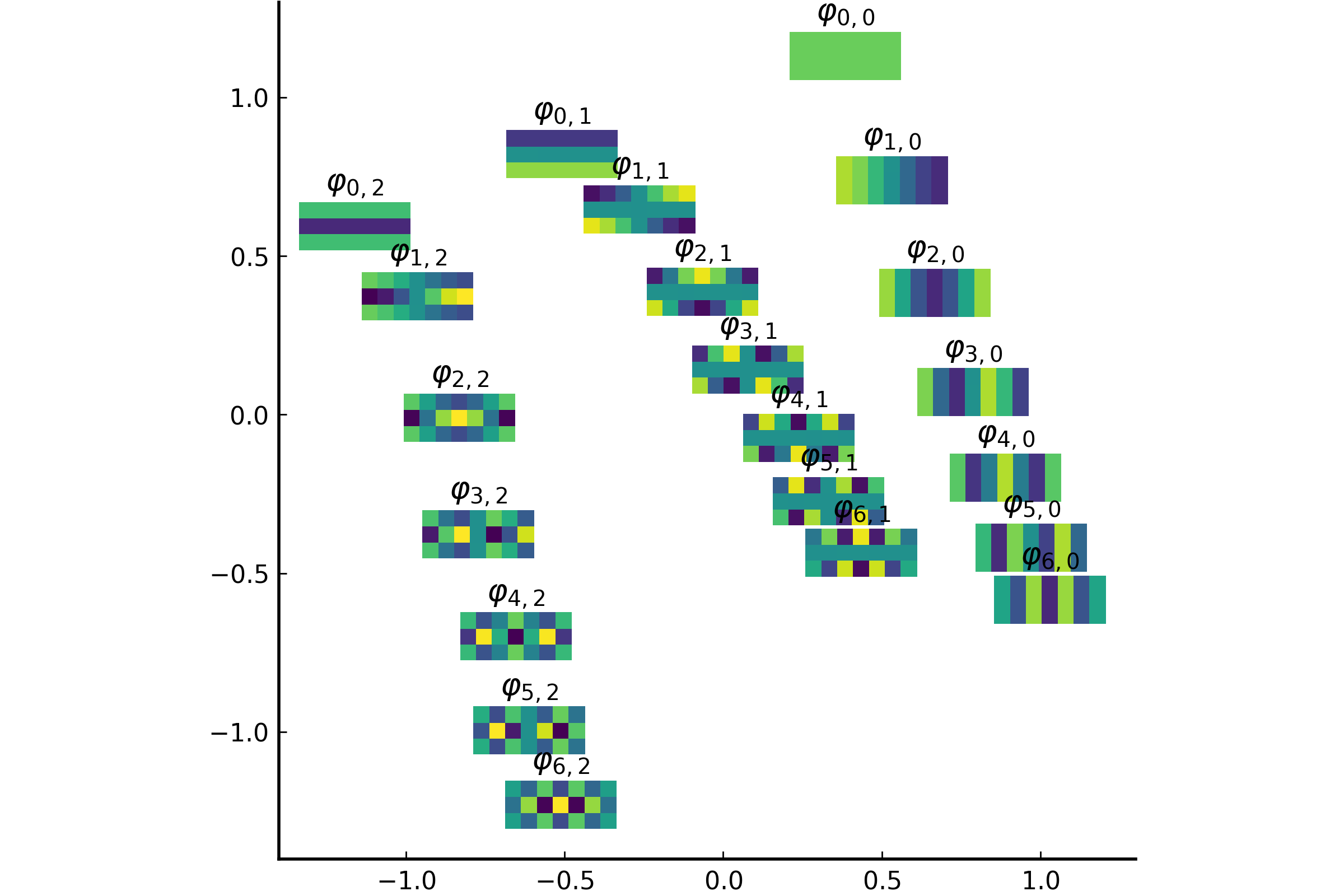
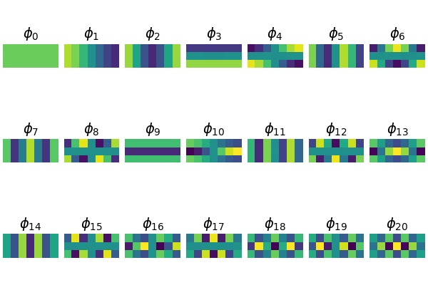
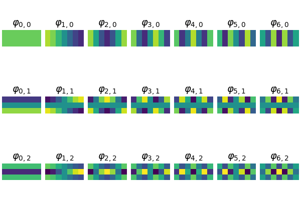
The integral operator $\mathcal{K}$ commutes with the Laplacian $\mathcal{L}) with the above nonlocal boundary condition. Consequently, the integral operator \(\mathcal{K}$ is compact and self-adjoint on $L^2(\Omega)$. Thus, the kernel $K(\boldsymbol{x},\boldsymbol{y})$ has the following eigenfunction expansion (in the sense of mean convergence): $$ K(\boldsymbol{x},\boldsymbol{y}) \sim \sum_{j=1}^\infty \mu_j \varphi_j(\boldsymbol{x})\overline{\varphi_j(\boldsymbol{y})}, $$ and $\{ \varphi_j \}_{j \in \mathbb{N}}$ forms an orthonormal basis of $L^2(\Omega)$.

It turned out that such eigenfunctions $\{\varphi_j\}$ satisfy the following peculiar extension to the outside of $\Omega$:

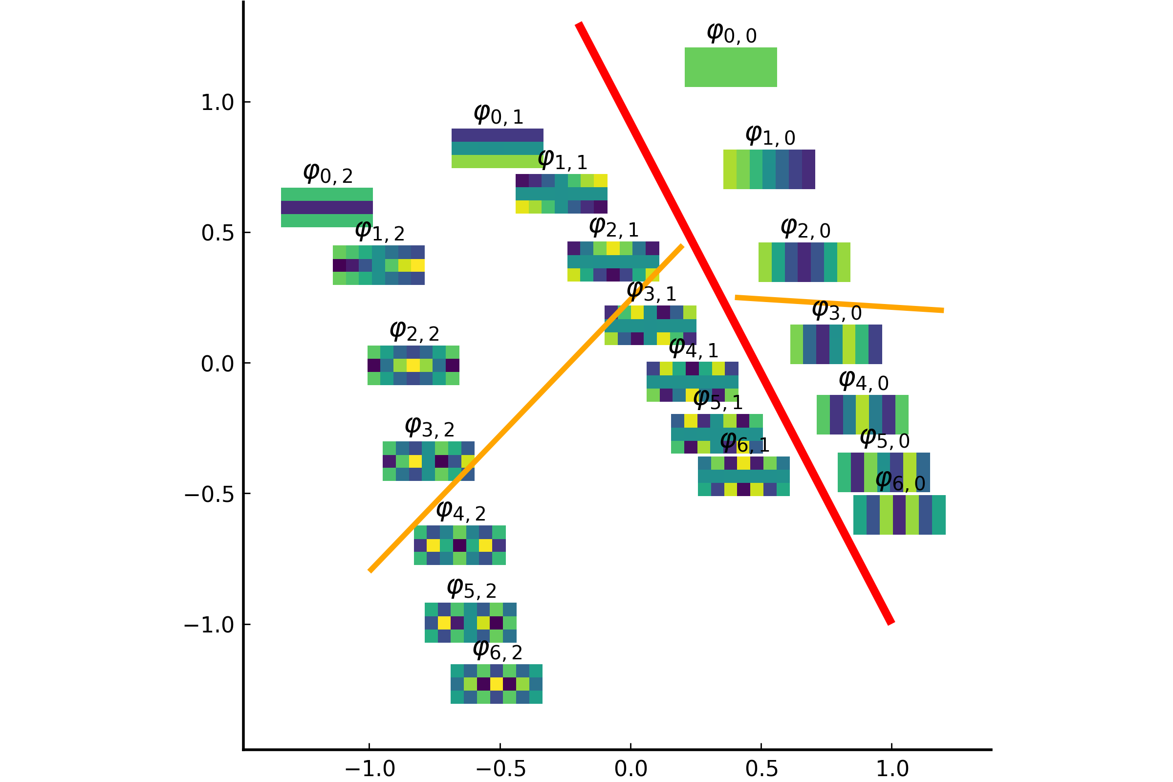
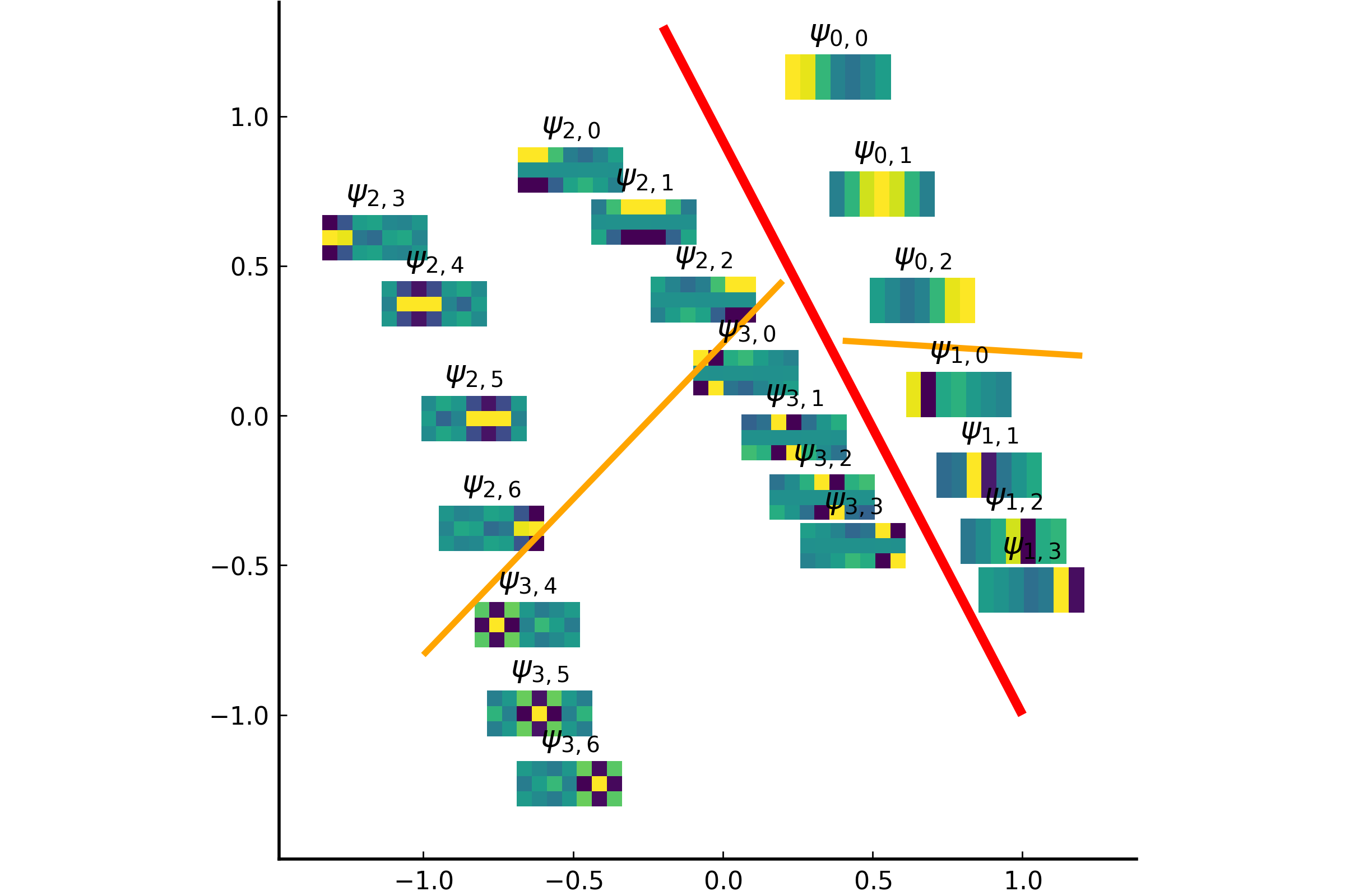
The eigenfunction $\varphi(\boldsymbol{x})$ of the integral operator $\mathcal{K}$ in the previous theorem can be $\color{orange}{\textit{extended}}$ outside the domain $\Omega$ and satisfies the following equation: $$ -\varDelta \varphi = \begin{cases} \lambda \, \varphi & \text{if $\boldsymbol{x} \in \Omega$}; \\ 0 & \text{if $\boldsymbol{x} \in \mathbb{R}^d\setminus\overline{\Omega}$} , \end{cases} $$ with the boundary condition that $\varphi$ and $\partial_\nu \varphi$ are continuous $\color{orange}{\textit{across}}$ the boundary $\partial \Omega$. Moreover, as $|\boldsymbol{x}| \to \infty$, $\varphi(\boldsymbol{x})$ must be of the following form: $$ \varphi(\boldsymbol{x}) = \begin{cases} \mathrm{const} \cdot | \boldsymbol{x} |^{2-d} + O(|\boldsymbol{x}|^{1-d}) & \text{if $d \neq 2$}; \\ \mathrm{const} \cdot \ln | \boldsymbol{x} | + O(|\boldsymbol{x}|^{-1}) & \text{if $d = 2$}. \end{cases} $$

It would be really nice if one could give physical interpretation to this problem: what is the physical phenomenon that is oscillatory inside $\Omega$ and is harmonic outside $\Omega$?
For the standard and simple domains, I could derive the eigenpairs of $\mathcal{K}$ explicitly. For example, for $d=1$ and $\Omega=(0,1)$, the above eigenvalue problem in the differential equation side becomes: $$ \begin{cases} - \varphi'' = \lambda \varphi, \quad x \in (0,1);\\ \varphi(0)+\varphi(1)=-\varphi'(0)=\varphi'(1). \end{cases} $$ The eigenpairs are:

$\lambda_0 \approx -5.756915$ is the unique root of $\tanh \frac{\sqrt{-\lambda_0}}{2} = \frac{2}{\sqrt{-\lambda_0}}$; $ \varphi_0(x) = A_0 \cosh \sqrt{-\lambda_0} (x-\frac{1}{2})$, where $A_0$ is a normalization constant;

$\lambda_{2m-1}=(2m-1)^2 \pi^2; \varphi_{2m-1}(x) = \sqrt{2} \cos(2m-1)\pi x, m=1,2,\ldots$;

$\lambda_{2m}$ is the root of $\tan \frac{\sqrt{\lambda_{2m}}}{2} = -\frac{2}{\sqrt{\lambda_{2m}}}$; $ \varphi_{2m}(x)=A_{2m} \cos \sqrt{\lambda_{2m}}(x-\frac{1}{2}), $ where $A_{2m}$ is a normalization constant, $m = 1, 2, \ldots$

These functions form an ONB of $L^2(0,1)$, which I never encountered before.
For the 2D unit disk, I got the following interesting results. The Laplacian eigenvalue problem becomes $$ \begin{cases} - \varDelta \varphi = \lambda \varphi, \quad \text{in $\Omega$}; \\ \displaystyle \partial_\nu \varphi \Big\vert_{\partial\Omega} = \frac{\partial\varphi}{\partial r} \Big\vert_{\partial \Omega} = - \frac{\partial \mathcal{H} \varphi}{\partial \theta} \Big\vert_{\partial \Omega}, \end{cases} $$ where $\mathcal{H}$ is the Hilbert transform for the circle, i.e., $$ \mathcal{H} f(\theta) := \frac{1}{2\pi} \mathrm{pv}\!\!\int_{-\pi}^\pi f(\eta)\cot\left( \frac{\theta-\eta}{2} \right) \, \mathrm{d}\eta \quad \theta \in [-\pi, \pi]. $$ Let $j_{k,\ell}$ is the $\ell$th zero of the Bessel function of order $k$, i.e., $J_{k}(j_{k,\ell})=0$. Then, $$ \varphi_{m,n}(r,\theta) = \begin{cases} J_m(j_{\textcolor{orange}{m-1},n} \, r) \binom{\cos}{\sin}(m\theta) & \text{if $m = 1, 2, \dots, \, n=1, 2, \ldots$}, \\ J_0(j_{0,n} \, r) & \text{if $m = 0, \, n = 1, 2, \ldots$}, \end{cases} $$ $$ \lambda_{m,n} = \begin{cases} j_{\textcolor{orange}{m-1},n}^2, & \text{if $m = 1, \ldots, \, n=1, 2, \ldots$}, \\ j_{0,n}^2 & \text{if $m = 0, \, n = 1, 2, \ldots$}. \end{cases} $$ Note that the Dirichlet-Laplacian eigenpairs are $\varphi_{m,n}(r,\theta) = J_m(j_{m,n}r) \binom{\cos}{\sin}(m\theta)$ and $\lambda_{m,n}=j_{m,n}^2$, $m=0, 1, \ldots, n=1, 2, \ldots$.

Laplacian eigenfunctions on an irregular domain should be useful for interactive image analysis, discrimination, interpretation, etc., in particular, medical image analysis, biometry, geophysical data assimilation, etc. Here, I want to discuss a particular application to analyze a stochastic process living on a domain $\Omega$. Typically, PCA/Karhunen-Loève Transform is used to analyze the samples (or realizations) of such a stochastic process. Note that PCA/KLT implicitly incorporate geometric information of the measurement location through data correlation; consequently, the PCA coordinates /KL expansion coefficients depend both the geometry of the domain and the statistics of the stochastic process. On the other hand, my Laplacian eigenfunctions use explicit geometric information through the harmonic kernel $K(\boldsymbol{x},\boldsymbol{y})$, and can decouple geometry/domain information and statistics of data; in other words, the statistics of the process is entirely encoded in the expansion coefficients while the geometric information is captured by the eigenfunctions.
Here is a demonstration. I used the "Rogues' Gallery" dataset again, but extracted only left and right eye regions (of 190 pixels). Then I computed the PCA/KL basis vectors using 72 randomly selected pairs of eyes and the Laplacian eigenfunctions of the eye region.

Note that all the KL basis vectors are simply linear combinations of the eyes in the training dataset. This is the reason why they all look like some variations of the actual eyes. On the other hand, these Laplacian eigenvectors are completely independent from the statistics of the eye training dataset; they only depend on the shape of the domain. Note also that they reveal the even and odd symmetry similar to cosines and sines in the conventional Fourier analysis. This property turns out to be decisive for certain applications such as the detection of "asymmetric" eyes. We can further see this effect in the following figure.

As we can observe from these figures, the KLT/PCA push more energy of the data into the top few coordinates than the Laplacian eigencoordinates. In terms of interpretability, however, the Laplacian eigenvectors are far more intuitive and give us an insight into the nature of this dataset. For example, we can see that there are several Laplacian eigencoordinates with high energy, e.g., the coordinates #7 and #13. If we check what these coordinates are in the Laplacian eigenvector figure, the eigenvector #7 correlates well with the iris in the eyes while the eigenvector \#13 indicates how wide the eyes are open. On the other hand, it is very difficult to do this type of analysis and interpretation with the KLT/PCA coordinates.
Note that my approach to computing the Laplacian eigenfunctions via diagonalization of the integral operator commuting with the Laplacian (after discretizing the domain) is computationally quite stable although it uses a dense matrix. In order to speed up the diagonalization of such a kernel matrix, one can fully utilize the celebrated Fast Multipole Method (FMM) thanks to my use of the harmonic kernel. My PhD student, Xiaodong "Allen" Xue, implemented this FMM-based algorithm and tested on a large scale data, which was of size $387924 \times 387924$; see his PhD dissertation for the details.

I presented my idea and preliminary results at the 13th IEEE Statistical Signal Processing Workshop held in Bordeaux, France in July 2005, and gave seminars on this subject at various places including academic institutions and industry in France, Japan, Switzerland, US. The journal version of this work was published in July 2008 in the journal Applied and Computational Harmonic Analysis.
My idea of using integral operators commuting with the Laplacians drew some attention from pure mathematicians to application domain experts. For the former, T. Sh. Kal'menov and his group in Kazakhstan have done many related works while the latter includes Faisal Beg who used it for his 3D hippocampus shape analysis for detecting early Alzheimer's disease and Tim DelSole who used it to compute the Laplacian eigenfunctions of the continental part and the oceanic part of the world separately for his climate data analysis. I also co-organized many minisymposia at various conference venues as well as two of 5 day workshops at IPAM in Feb. 2009 and BIRS in March 2015, all of which dealt with Laplacian eigenfunctions and their applications; see my Conferences & Workshops Resource Page for the details.

I want to describe some unresolved issues in my approach of using the commuting integral operator. In October, 2012, my collaborator Lotfi Hermi invited me to give a talk at the special session on "The Ubiquitous Laplacian: Theory, Applications, and Computations" at the AMS Sectional Meeting held in Tucson, AZ. In the evening of the first day, there was a party at Lennie Friedlander's house, and I talked with Mark Ashbaugh about my approach, and in particular, my eigenfunctions that are harmonic outside of the domain $\Omega$. Mark pointed out that my eigenfunctions may be related to the so-called Von Neumann-Krein Laplacian, and suggested that I study further. I worked on this project and learned various extensions through the book Unbounded Self-adjoint Operators on Hilbert Space written by Konrad Schmüdgen. As of today, I only partially figured out this problem, and I presented my understanding at the SIAM Annual Meeting in 2013. In essence, in the case of 1D, i.e., $\Omega=(0,1)$, the boundary conditions of the Von Neumann-Krein Laplacian is $\varphi'(0)=\varphi'(1)=\varphi(1)-\varphi(0)$, and the first two eigenfunctions are the constant and linear functions both corresponding to the eigenvalue 0. In higher dimension, the boundary condition of the Von Neumann-Krein Laplacian becomes $\partial_\nu \varphi(\boldsymbol{x}) = \partial_\nu \mathcal{P}\left[ \varphi \vert_{\partial \Omega} \right](\boldsymbol{x})$ for $\boldsymbol{x} \in \partial\Omega$, where $\mathcal{P}\left[ \varphi \vert_{\partial \Omega} \right]$ is a harmonic function in $\Omega$ with the Dirichlet boundary data are given (or set) by $ \varphi \vert_{\partial\Omega} $. See my presentation slides, in particular, page 37-41, for the details.
Then, in December 2014, I was invited to give my presentation on this subject at the Analysis & PDE Seminar at UC Berkeley. There, Alberto Grünbaum asked me what is the physical interpretation of the nonlocal boundary condition above, i.e., $\varphi(0)+\varphi(1)=-\varphi'(0)=\varphi'(1)$ when one considers a random walk on $[0,1]$. As is well known, the Dirichlet and Neumann boundary conditions correspond to the absorbing and reflecting boundaries in the context of random walk. Again, as of today, I have not completely resolved how to interpret my nonlocal boundary condition, and have been collaborating with Lotfi Hermi on this subject.
Finally, my integral operator has a link with the Volterra operator, which I found out by checking the famous book Introduction to the Theory of Linear Nonselfadjoint Operators in Hilbert Space written by Israel Gohberg and Mark Krein. For the 1D case, they discussed the iterated Volterra integral operator on $L^2(0,1)$ on pages 240-241: $$ A f(x) := \int_x^1 f(y) \, \mathrm{d}y \Longrightarrow A^2 f(x) = \int_x^1 (x-y) f(y) \, \mathrm{d}y, $$ which was decomposed into the real and imaginary parts: $$ \begin{eqnarray*} (A^2)_R f & := & \frac{1}{2} (A^2 + A^{2*}) = - \frac{1}{2} \int_0^1 |x - y| f(y) \, \mathrm{d}y \, ; \\ (A^2)_I f & := & \frac{1}{2\mathrm{i}} (A^2 - A^{2*}) = \frac{1}{2\mathrm{i}} \int_0^1 (x - y) f(y) \, \mathrm{d}y. \end{eqnarray*} $$ As one can see, $(A^2)_R$ is exactly the same as my $\mathcal{K}$ for $\Omega=(0,1)$. Is this simply a coincidence? What is the situation in higher dimensions? I do not know yet. However, my instinct tells me there is a deeper connection between my integral operators and such Volterra operators. See my presentation slides, in particular, page 35-36, for more information.

In addition, Lotfi Hermi and I further studied the generalization of my 1D integral operator with the kernel function $|x-y|^\rho, 0 \lt \rho \leq 1$ on the 1D interval $\Omega = (-a,a)$. We could prove the existence, uniqueness, and simplicity of a negative eigenvalue for this class of integral operators. We also provided two different ways of producing recursive formulas for the Rayleigh functions—recursion formulas for power sums—of the eigenvalues of this integral operator for $\rho=1$, providing means of approximating this negative eigenvalue. More precisely, we proved the following theorem:

Let $\{ \lambda_n \}_{n=0}^\infty$ be the eigenvalues of the nonlocal boundary value problem associated with the harmonic kernel $K(x,y)=-|x-y|/2$ on $\Omega=(0,1)$. Let $K_p(x,y)$ be the $p$th iterated kernel of $K(x,y)$. Then, we have $$ \sum_{n=0}^\infty \frac{1}{\lambda^p_n} = \int_0^1 K_p(x,x) \, \mathrm{d}x = \frac{1}{4^p} \left( S_{2p} + \frac{(-1)^p}{\alpha^{2p}} \right) + \frac{4^p-1}{2 \cdot (2p)!} |B_{2p}|, $$ where $\displaystyle S_{2p} = \sum_{m=1}^\infty \left( \frac{4}{\lambda_{2m}} \right)^p $, $\alpha \approx 1.19967864$ is a unique root of $\alpha = \coth \alpha$, and $B_{2p}$ is the Bernoulli number, which is defined via the generating function: $\displaystyle \frac{x}{\mathrm{e}^x-1} = \sum_{n=0}^\infty \frac{B_n}{n!}x^n $. Moreover, $S_{2p}$ satisfies the following recursion formula: $$ \sum_{\ell=1}^{n+1} \frac{(-1)^{n-\ell+1} \left( 2\left(n-\ell+1\right)-1\right)}{\left( 2\left(n-\ell+1\right)\right)!} \left\{ S_{2\ell} + \frac{(-1)^\ell}{\alpha^{2\ell}} \right\} = \frac{(-1)^n}{2(2n)!}. $$

Note that setting $p=1$ in the above formula, we have $\displaystyle \sum_{n=0}^\infty \frac{1}{\lambda_n} = 0$. Our results were published in July 2018 in the journal Applied and Computational Harmonic Analysis.

Graph Laplacians, Phase Transitions, and Dendritic Trees
While I was working on the integral operators commuting with Laplacians on general shape domains, I attended a UC Davis Vision Science Retreat in March 2007, and heard Leo Chalupa describe his project on morphological analysis of dendritic trees of retinal ganglion cells (RGCs) of a mouse. Vision scientists like him want to understand how the morphological properties of dendrite patterns of RGCs relate to the functional types of these cells. Although such classification of neurons should ultimately be done on the basis of molecular or genetic markers of neuronal types, it has not been forthcoming. Hence, neuronal morphology has often been used as a neuronal signature that allows one to classify a neuron into different functional cell types. The state of the art procedure is still quite labor intensive and costly: automatic segmentation algorithms to trace dendrites in a given 3D image obtained by a confocal microscope only generate imperfect results due to occlusions and noise; moreover, one has to painstakingly extract many morphological and geometrical parameters (e.g., somal size, dendritic field size, total dendrite length, the number of branches, branch angle, etc.) with the help of an interactive software system. In fact, 14 morphological and geometric parameters were extracted from each cell in Leo's project. According to his associate, Julie Coombs, it would take roughly several hours to process a single cell from segmentation to parameter extraction!
I was intrigued by his project; actually I immediately thought that the Laplacian eigenvalues and eigenfunctions would be useful to analyze morphological properties of such dendritic trees. Around this time, I was studying the graph Laplacians and their relationship with the discretized version of my integral operators commuting with general shape domain in the Euclidean space, and studied many papers and books included those by Fan Chung, Russell Merris, Hajime Urakawa, and so forth. Given a graph $G=G(V,E)$, where $V$ and $E$ are the vertex set and edge set of $G$, respectively, with $|V|=n$, $|E|=m$, the graph Laplacian matrix is defined as $L(G) := D(G)-A(G) \in \mathbb{R}^n$ where $A(G)=(a_{ij})$ is the adjacency matrix describing the connectivity of the nodes of $G$ and $D(G) := \mathrm{diag}(d_1, \ldots, d_n)$ is the degree matrix where $d_i=\sum_{j=1}^n a_{ij}$ is a degree of node $i$. The matrix $L(G)$ can be viewed as a finite difference approximation of the negative Laplacian $-\varDelta$ on $G$. Soon, I discovered that for a path graph consisting of $n$ nodes, often denoted by $P_n$, its graph Laplacian matrix is the following tridiagonal matrix, $$ \underbrace{ \begin{bmatrix} 1 & -1 & & & & \\ -1 & 2 & -1 & & & \\ & -1 & 2 & -1 & & \\ & & \ddots & \ddots & \ddots & \\ & & & -1 & 2 & -1 \\ & & & & -1 & 1 \end{bmatrix}}_{L(G)} = \underbrace{\begin{bmatrix} 1 & & & & & \\ & 2 & & & & \\ & & 2 & & & \\ & & & \ddots & & \\ & & & & 2 & \\ & & & & & 1 \end{bmatrix}}_{D(G)} - \underbrace{\begin{bmatrix} 0 & 1 & & & & \\ 1 & 0 & 1 & & & \\ & 1 & 0 & 1 & & \\ & & \ddots & \ddots & \ddots & \\ & & & 1 & 0 & 1 \\ & & & & 1 & 0 \end{bmatrix}}_{A(G)} $$ and its eigenvectors are nothing but the DCT Type II, which is the backbone of the JPEG image compression standard! Actually, the eigenvalues are $\lambda_k = 4 \sin^2(\pi k / 2n)$, $k=0, 1, \dots, n-1$ whereas the eigenvectors are $\boldsymbol{\phi}_k(\ell) = a_{k;n} \cos(\pi k(\ell+1/2)/n)$, $k, \ell =0, 1, \dots, n-1$, where $a_{k;n}$ is a normalization constant so that $\|\boldsymbol{\phi}_k\|_2 = 1$. See a very well written paper by Gilbert Strang to see subtle differences in boundary conditions and grid discretizations lead to various types of DCTs. By now, this correspondence is a well-known fact, but I believe I was one of the first to point out this fact already in Feb. 2009, presented at the 5-day IPAM workshop on "Laplacian Eigenvalues and Eigenfunctions: Theory, Computation, Application," which I co-organized with Peter Jones and Denis Grebenkov. The actual publication including this fact appeared later in 2011 in the RIMS Kôkyûroku.
I got excited about this discovery, and I started examining the eigenpairs of the graph Laplacian matrix of each dendritic tree after my PhD student, Ernest Woei, converted the dendritic tree dataset obtained from Julie Coombs to actual graphs consisting of vertices/nodes and edges. Actually, we converted them literally to "trees" by replacing a cycle representing a soma into a single node. After computing the Laplacian eigenvalues of 130 dendritic trees of RGCs, we computed four features based on such eigenvalues: 1) the lower bound of the number of the pendant neighbors (i.e., those nodes adjacent to the pendant/leaf nodes); 2) the Wiener index; 3) the number of eigenvalues larger than 4; and 4) the upper bound of the isoperimetric number (a.k.a. the Cheeger constant). Note that Features 1 to 3 should be normalized by the number of the total nodes in each tree to make these features less dependent on how the dendrite arbors are sampled. Our visualization of these four features allows us to separate a group of sparsely and widely distributed dendritic trees from that of densely packed dendritic trees; see our published short article for the details.
While I was conducting the analysis, I noticed quite a peculiar behavior of the Laplacian eigenvalues of these dendritic trees when each edge weight is 1.

As one can see from the above figure (b), the eigenvalue distribution has a nice bell-shape curve starting at the eigenvalue 0, and then around the eigenvalue 4, there is a sudden jump, followed by several eigenvalues greater than 4. Hence, I wanted to see what happens in the eigenvectors before and after the eigenvalue 4. The below are such plots.

(a) $\varphi_{1141}$ corresponding to $\lambda_{1141}=3.9994$

As one can see, this is a kind of phase transition phenomenon: the eigenfunctions corresponding to the eigenvalues below 4 are semi-global oscillations (like Fourier cosines) over the entire dendrites or one of the dendrite arbors while those corresponding to the eigenvalues above 4 are much more localized (like wavelets) around junctions/bifurcation nodes. Each dendritic tree I examined exhibited this phenomenon. Hence, I wanted to know know why such localization/phase transition occurs on dendritic tree graphs. It took for a while, but thanks to the help from Yuji Nakatsukasa, we found why this happens with a proof, which I first reported at the minisymposium on "Harmonic Analysis on Graphs and Networks" at International Congress on Industrial and Applied Mathematics (ICIAM), held in Vancouver, Canada, in July 2011, which I co-organized with Mauro Maggioni. Subsequently, we published the details in the journal Linear Algebra & its Applications in April 2013. The key was the discriminant of a quadratic equation describing the graph Laplacian eigenvalue problem along each branch of a dendritic tree, say, the first branch containing $n_1$ nodes. This leads to the following recursion formula: $\phi_{j+1} +(\lambda-2)\phi_j + \phi_{j-1} =0$, $j=2,\ldots,n_1$ with the appropriate boundary condition. Then, its characteristic equation is simply $r^2 + (\lambda - 2)r + 1 = 0$, and the general solution for the above recursion formula can be written as $\phi_j = A r^{j-2} + B r^{j-2}$, $j=2,\ldots,n_1+1$, where $r_1, r_2$ are the roots of this characteristic equation, and $A, B$ are appropriate constants determined by the boundary condition. Now, the discriminant of the characteristic equation is $ D(\lambda) := (\lambda-2)^2 - 4 = \lambda(\lambda-4)$. Hence if $0 \leq \lambda \lt 4$, then $r_1, r_2 \in \mathbb{C}$, which give us the oscillatory solution while if $\lambda \gt 4$, we can show $r_1 \lt -1 \lt r_2 \lt 0$, which leads to the more concentrated solution. In our paper, we proved not only the above but also various interesting observations we made on the spectral behavior of more general graphs including (but not limited to): 1) the number of the eigenvalues greater than 4 is bounded from above by the number of nodes whose degree is greater than 2; 2) if a graph contains a branching path, then the eigencomponents for $\lambda \gt 4$ decay exponentially from the branching vertex toward the leaf. In addition, I tried to answer the following question: "Can a simple and connected graph, not necessarily a tree, have eigenvalues equal to 4?" The answer is a clear "Yes." For example, a regular finite lattice graph in $\mathbb{R}^d$, $d \gt 1$, which is simply the $d$-fold Cartesian product of $P_n$ with itself. Such a lattice graph has repeated eigenvalue 4. In fact, each eigenvalue and the corresponding eigenvector of such a lattice graph can be written as $$ \begin{eqnarray*} \lambda_{j_1, \dots, j_d} &=& 4 \sum_{i=1}^d \sin^2\left( \frac{j_i \pi}{2n} \right) \\ \phi_{j_1, \dots, j_d}(x_1, \dots, x_d) &=& \prod_{i=1}^d \cos \left( \frac{j_i \pi (x_i+\frac{1}{2})}{n} \right), \end{eqnarray*} $$ where $j_i, x_i \in \mathbb{Z}/n\mathbb{Z}$ for each $i$, as shown by Burden and Hedstrom. Now, determining $m_G(4)$, i.e., the multiplicity of the eigenvalue 4 of this lattice graph, turns out to be equivalent to finding the number of the integer solutions $(j_1, \dots, j_d) \in (\mathbb{Z}/n\mathbb{Z})^d$ to the following equation: $$ \sum_{i=1}^d \sin^2\left( \frac{j_i \pi}{2n} \right) = 1. $$ For $d=1$, there is no solution anyways since the eigenvalue never reaches 4. For $d=2$, it is easy to show that $m_G(4) = n-1$ by direct examination of the above equation using some trigonometric identities. For $d=3$, $m_G(4)$ behaves in a much more complicated manner, which is deeply related to number theory. We expect that more complicated situations occur for $d > 3$. I asked this question to Terry Tao when both of us attended the Joint Birthday Conference of Coifman-Jones-Rokhlin at Yale in June 2012. He later told me that this problem would be quite difficult to solve, but may be related to a paper he wrote earlier. Later on, my colleague, Greg Kuperberg pointed out that this may be related to the so-called Euler's totient function. To date, I do not know if this problem can be completely resolved.
On the other hand, it is clear from the above eigenvector formula that the eigenvectors corresponding to the eigenvalues greater than or equal to 4 on such lattice graphs cannot be localized or concentrated on those vertices whose degree is higher than 2 unlike the tree case.
I am very satisfied by these results. In some sense, I was lucky because if I had converted the dendritic trees to weighted graphs whose edge weight represents either distance between sampling points or its inverse, then I could not have observed the universal threshold eigenvalue 4: it would have varied depending on a dendritic tree. Our paper also induced others to study such phase transition phenomena on "uniform" trees consisting of concatenated starlike trees. Now, whether our results have any physiological explanations or suggest importance of branching nodes, is not clear to me at this point. In any case, many such eigenvector localization phenomena have been reported: Anderson localization, "scars" in quantum chaos, etc. I also want to point out an interesting related work for more general setting and for application in numerical linear algebra by my colleague, Thomas Strohmer and his collaborators.
I want to emphasize that eigenvectors corresponding to high eigenvalues are quite sensitive to topology and geometry of the underlying domain and cannot really be viewed as high frequency oscillations unless the underlying graph is a simple unweighted path or cycle. This observation strongly motivated me to construct wavelets and wavelet packets naturally adapted to the graph setting, as I describe later.
After the above work, Ernest Woei and I developed a "tree simplification" procedure, which reduces the number of nodes and edges of a given tree without changing its topological information. Our motivation for developing this procedure was to reduce computational costs of graph Laplacian eigenvalues of such trees. When we applied this procedure to dendritic trees and computed their graph Laplacian eigenvalues, we observed two "plateaux" (i.e., two sets of multiple eigenvalues) in the eigenvalue distribution of each such simplified tree. This again spiked my interest, and I wanted to understand why such plateaux occur. We could explain such plateaux can occur in a more general graph if it satisfies a certain condition; and identify these two eigenvalues specifically as well as the lower bound to their multiplicity. More precisely, we proved the following theorem:

Let $G(V,E)$ be a simple, connected, undirected, and unweighted graph with $n=|V|$. Let $\theta = \frac{3-\sqrt{5}}{2}$ and $\theta^* = \frac{3+\sqrt{5}}{2}$. Let $\tau$ be the difference between: 1) the number of degree 2 nodes each of which is adjacent to a leaf node and a node whose degree is 3 or higher; and 2) the number of the latter high degree nodes. Suppose $\tau \geq 1$, then $$ m_G(\theta) = m_G(\theta^*) \geq \tau . $$ In other words, the multiplicity of the graph Laplacian eigenvalues $\theta$ and that of $\theta^*$ are the same and at least $\tau$.

Our results were published in Linear Algebra & its Applications in September 2015. This paper certainly drew attention from a group of mathematicians. In our paper, we also stated our conjecture: the difference between the number of the specially-qualified pendant vertices and their neighbors is bounded from above by the multiplicity of a certain graph Laplacian eigenvalue. This conjecture was proved in August 2016, and the generalized version of our conjecture for signless Laplacians has been also proved in October 2016.

Hierarchical Graph Laplacian Eigen Transform
I was fortunate to have Jeff Irion as my PhD student who started working with me in Winter 2011. In April 2011, he was awarded the prestigious National Defense Science and Engineering Graduate (NDSEG) Fellowship. Around this time, I wanted to develop wavelets and wavelet packets for graphs and networks. Time-honored harmonic analysis tools such as Fourier and wavelet transforms have been the 'crown jewels' for examining regularly-sampled data. These tools have a wide range of applications, e.g., data compression, image analysis, and statistical signal processing. So, it was my natural desire to lift those classical tools to the graph setting, and I assigned this project to Jeff as his PhD research.
After both of us reviewed and studied the wavelet-like transforms for the graph setting that had been proposed by then, Jeff initially tried to develop Haar-like transform for a graph by hierarchically and recursively bipartitioning it using the Fiedler vector, $\boldsymbol{\phi}_1$, the Laplacian eigenvector of each subgraph corresponding to the smallest nonzero eigenvalue $\lambda_1$. Such Fiedler vectors play duals roles to: 1) partition subgraphs; and 2) the Haar-like function after appropriate binarization. While we examined and developed his algorithm, I first realized that we should consider not only the first two Laplacian eigenvectors of each subgraph but all of them to generate a basis dictionary, which turned out to be a complete generalization of the hierarchical block DCT dictionary for the graph setting: if an input graph is an unweighted and undirected path graph, then the HGLET exactly coincides with the regular block DCT dictionary developed on an input 1D signal whose samples are represented by the path graph. We named this basis dictionary generating procedure Hierarchical Graph Laplacian Eigen Transform (HGLET), and conducted a large number of numerical experiments. The following figure shows four basis vectors $\{\boldsymbol{\phi}^j_{k,l}\}$ in the HGLET dictionary computed on the popular Minnesota road network with $n=2636$ (obtained through the courtesy of David Gleich), where $j, k, l$ represent spatial scale, region index, and eigenvector index ($\approx$ frequency), respectively.

I first presented our results at the special session on wavelets at the Japan SIAM Annual Meeting, which was held in Fukuoka, Japan, in September 2013. This gave us an opportunity to publish our short paper in the journal JSIAM Letters, which appeared in May 2014. Although it is a short paper, I am very proud of this paper since we won the JSIAM Letters Best Paper Award in September 2016!

Generalized Haar-Walsh Transform and Its Extension
In late 2013, Jeff and I were working on the Haar-like transform for the graph setting using the first two Laplacian eigenvectors of each subgraph in the hierarchical partition tree of an input graph, which was also published as a section in our HGLET paper. However, that was not really satisfactory since it was not a true generalization of the Haar-Walsh wavelet packet dictionary. Then, Jeff managed to track the average and difference operations of data on subgraphs using the tags, which encodes a sequence of such operations via binary digits. Another important issue was the fact that the number of nodes $|V|=n$ cannot be assumed to be a dyadic integer. Hence, when the hierarchical bipartitioning is applied to a given graph, we need to allow a single node subgraph to go down the partition tree without further splitting it; see the following figure (a) for the details, which shows the hierarchical bipartition tree of the $P_6$ path graph and the associated basis vectors. This way of organizing the basis vectors in this dictionary is called a "coarse to fine" (c2f) dictionary since it starts with the global basis vectors in the root node and ends with the unit impulse (i.e., extremely localized) basis vectors at the leaf nodes. The true Haar-Walsh wavelet packet dictionary, however, should be arranged in the "fine to coarse" (f2c) manner. We could achieve such an rearrangement using the tag, which is shown in the following figure (b) for $P_6$.

In the above figures, the indices $j, k, l$ in the basis vector $\boldsymbol{\psi}^j_{k,l}$ represent its spatial scale, region index, and tag, respectively. The black, red, and blue basis vectors correspond to the scaling (or father), the Haar (or mother), and the Walsh vectors, respectively. Because of this hierarchical tree structure, we can apply the best-basis algorithm and its relatives as I described above to select the most appropriate basis from this basis dictionaries. Note that the Haar basis can be chosen as the best basis for certain graph signals only using the f2c dictionary; the best-basis algorithm cannot choose the Haar basis from the c2f dictionary. The above figures can explain this situation. Also, this means that we can select the best of the two best bases selected from these two dictionaries. Note also that the GHWT basis vectors are still "blocky", yet they are not "binary" valued: the constant levels depend on the number of nodes of subgraphs that support the basis vectors.
We named these basis dictionaries the "Generalized Haar-Walsh Transform" (GHWT). The following figures show some of the GHWT basis vectors computed on the Minnesota road network.

I presented our results at at the 18th IEEE Statistical Signal Processing Workshop held in Gold Coast, Australia, in July 2014, and published the conference proceeding paper. I also gave a tutorial on Laplacian eigenfunctions (including those on graphs) in that workshop.
Later on in 2015, I was invited to give a keynote talk at at the SPIE Conference on Wavelets & Sparsity XVI, in San Diego, August 2015, which summarizes our effort of lifting conventional time-frequency analysis tools to the graph setting and appeared in the Proceedings of SPIE in September 2015. Our numerical results shown in this paper drew attention of Stefan Steinerberger, who pointed out these to Hau-tieng Wu, who subsequently wrote an interesting paper with his collaborators in early 2020, which conjectures that the hierarchical spectral bipartitioning of a general connected domain in $\mathbb{R}^2$ other than an isosceles right triangle via the Fiedler vector of the 1-Laplacian eventually tend to generate a set of rectangles. Soon, the JSIAM invited me to write an article on applied harmonic analysis on graphs and networks (in Japanese) for their flagship journal, Bulletin of the Japan Society for Industrial and Applied Mathematics. The final version appeared in September 2015 and won the JSIAM Best Author Award in September 2016!

In early 2015, I got interested in analyzing matrix-form datasets such as term-document matrices and spatiotemporal measurements recorded by sensor networks, etc., using our tools, in particular, the GHWT. Of course, there were many works on matrix data analysis in general, but less so using harmonic analysis; the exception was the work by Raphy Coifman and Matan Gavish who used the Haar-like transform on rows and columns of a given matrix, which influenced my thinking. By mid 2015, Jeff and I developed a good strategy to do such matrix data analysis using the GHWT. Let me explain our work using an example of a particular term-document matrix. Here, the rows of such a matrix correspond to words and the columns correspond to documents, and matrix entry $a_{ij}$ is typically the (relative) frequency with which word $i$ appears in document $j$. In the case that the documents are journal articles from different fields, one would expect the prevalence and absence of certain words to be relatively consistent across documents from within each field. Such matrices are quite different from usual images and photographs. In fact, they are often more like shuffled and permuted images, possessing no spatial smoothness or coherency in general. Yet, those rows and columns are interrelated, and thus the rows of the matrix can tell us about the underlying structure of the columns, and vice versa. But how can we do that? Our GHWT now come to our rescue. This allows us to discover, learn, and exploit hidden dependency and geometric structure in the matrix data in an innovative way. Here is our strategy:

Apply spectral co-clustering to a given matrix in order to recursively bipartition its rows and columns
Analyze row vectors of the input matrix using the GHWT dictionaries based on the column partitions and extract the basis that most sparsifies its column representation, i.e., the column best basis
Repeat Step 2 with interchanging columns and rows to extract the row best basis
Expand the input matrix with respect to the tensor product of the column and row best bases
Analyze the expansion coefficients for a variety of tasks, e.g., compression, classification, etc.

In Step 1, the spectral co-clustering method, initially developed by Inderjit Dhillon in 2001, is recursively applied to an input matrix to organize its rows and columns. Given a nonnegative data matrix $A$, Dhillon's method treats its rows and columns as the two sets of nodes in a bipartite graph, where matrix entry $a_{ij}$ is the edge weight between the node for row $i$ and the node for column $j$.

The figure in the left illustrates a small scale example. This matrix consists of 5 words on 8 documents where the nonzero entries are indicated by the $\bullet$ symbol in the matrix shown on the left subfigure. Using the Dhillon's spectral co-clustering algorithm, this matrix is partitioned into two sub-bipartite graphs via the Fiedler vector of the initial bipartite graph.

Here is a real example: the term-document matrix consisting of 1042 columns representing documents obtained from the Science News website and 1153 rows representing preselected most relevant words. Each document belongs to one of the eight categories ranging from Anthropology to Physics.

This shows that both words and documents are embedded in the same Euclidean space using the spectral co-clustering! At the left side of the boomerang shape cluster, a majority of documents are of Astronomy (blue points) and the related words (e.g., extrasolar) are clustered closely to those documents while the right side of the boomerang mainly consists of Medical Science documents (red points) and the related words (e.g., tamoxifen). The following figures demonstrate the power of our strategy.

The above figure (b) shows the reordered matrix using our algorithm; the total number of orthonormal bases searched via their algorithm exceeds $10^{370}$. It is reassuring to see that the resulting best basis does in fact sparsify the input matrix nicely. However, the fine scale information may be too much emphasized in the original algorithm, which may be sensitive to "noise." More robust and useful information is contained at the medium scale coefficients in this matrix. To emphasize such coefficients, one possibility is to weight all the coefficients in the GHWT dictionaries depending on the size of the subgraphs so that the magnitude of the finer coefficients become bigger, which discourages the best basis algorithm from selecting fine scale subgraphs. This new best basis sparsifies $A$ less than before, yet well captures information on intermediate scales as shown below. Figure (c) shows the partition pattern of the column best basis: the vertical axis indicates the scale information from the top (the coarsest) to the bottom (the finest) whereas the horizontal axis indicates the reordered column indices. In this figure, two coarse scale blocks stand out; one of them is marked with the red circle. Figure (d) shows the column best basis vectors corresponding to the coefficients marked by the red circle in Figure (c) whose support corresponds to 51 documents with 48 belonging to Astronomy. The titles of the remaining three turn out to be the following:

"Old Glory, New Glory: The Star-Spangled Banner gets some tender loving care" [Anthropology; on the preservation of the Star-Spangled Banner (flag) using the space-age technology]

"Snouts: A star is born in a very odd way" [Life Sciences; on star-nosed moles]

"Gravity tugs at the center of a priority battle" [Math/CS; on the priority war on the discovery of gravity between Newton, Halley, and Hooke]

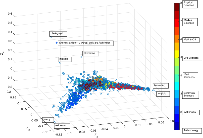
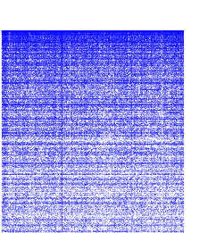
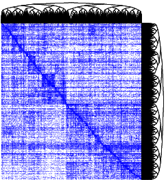
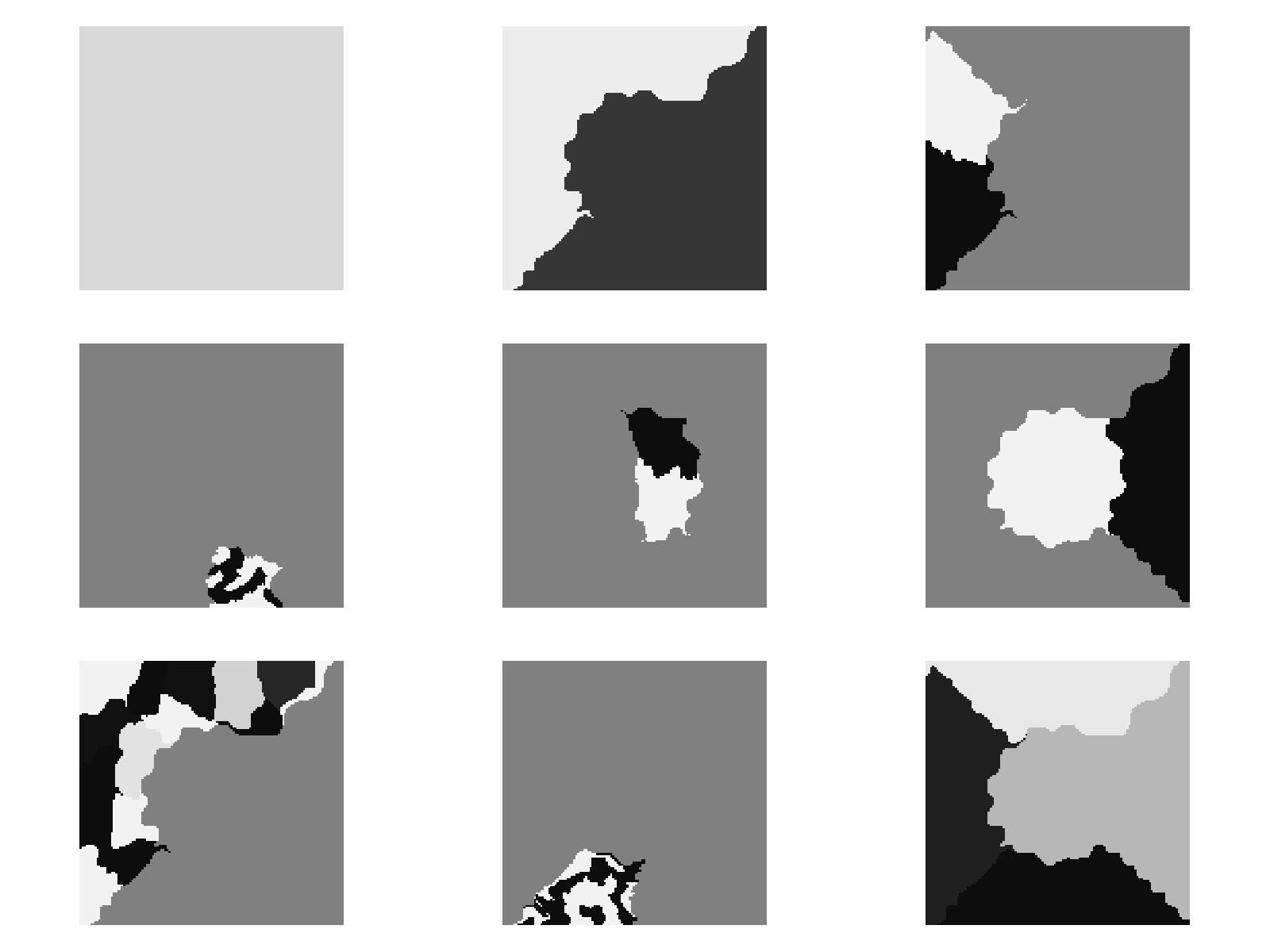
These three articles are picked out along with the Astronomy articles because they contain some astronomical keywords as one can see. Similarly, one can analyze another coarse block in Figure (c), which supports 62 documents: 56 of which are in Medical Sciences and the remaining six are non-medical articles that just happen to contain medical terms.
These results are based on the examination of the particular best basis vector and the corresponding coefficients at one intermediate scale. I think that our approach can further advance the state of clustering and classification of documents by linking information at multiple scales. I envision that these tools will be useful for finding "patterns" hidden in unorganized massive datasets of various kinds.
I presented our results at the 2016 IEEE 26th International Workshop on Machine Learning for Signal Processing (MLSP) held in Vietri sul Mare, Salerno, Italy, in September 2016, and the conference proceeding paper was published soon after that.

In Summer 2016, I wanted to extend our GHWT significantly by following the idea of my friends, Christoph Thiele and Lars Villemoes originally proposed back in 1996 for the regular dyadic lattice case. Their algorithm is to find the best basis for efficiently representing a given (non-graph) signal among the ONBs of $\mathbb{R}^n$ consisting of discretized rescaled Walsh functions, which are constructed by simultaneously partitioning time and frequency domain information. Yet $n$, the length of the signal, must be a dyadic integer in their algorithm. Together with my PhD student, Yiqun Shao, I substantially extended our GHWT, and proposed the extended Generalized Haar-Walsh Transform (eGHWT). The eGHWT and its associated best-basis selection algorithm for graph signals will significantly improve the performance of the previous GHWT with the similar computational cost, $O(n \log n)$ where $n$ is the number of nodes of an input graph. Our new eGHWT also simultaneously considers the graph domain split and "frequency" (or "sequency") domain split of an input graph signal, but $n$ does not have to be dyadic. It is quite satisfying to see that the eGHWT reduces to the original time-frequency adapted Haar-Walsh wavelet packets of Thiele and Villemoes if the input graph is a regular lattice graph consisting of a dyadic number of nodes for each direction. This transform will allow us to deploy the modified best-basis algorithm that can select the best ONB for a task at hand (e.g., efficient approximation, denoising, etc.) among a much larger collection ($\gt 0.618 \cdot (1.84)^n$) of ONBs than the GHWT dictionaries would provide ($\gt (1.5)^n$). For a large $n$, this difference is significant; even for the quite modest case of $n=1024$, the conventional GHWT/best-basis algorithm would search through approximately $10^{181}$ ONBs whereas our new eGHWT/best-basis algorithm could search the best one among staggering $10^{272}$ possible ONBs.
Let me explain how the eGHWT differ from the original GHWT using a very simple graph signal $\boldsymbol{f} = [2,-2,1,3,-1,-2]^{\scriptstyle{\mathsf{T}}}$ defined on $P_6$.

The eGHWT best basis in the above figures are indicated by red. As you can see, this combination of the basis vectors cannot be chosen by the original GHWT best-basis algorithm operated within the c2f and f2c dictionaries. Note also that these red basis vectors are orthogonal to each other.
Now, let me show you our analysis of a real graph signal: the vehicular traffic volume data on the Toronto road network which contains the most recent 8 peak-hour vehicle volume counts collected at intersections where there are traffic signals. The data was typically collected between the hours of 7:30am and 6:00pm, over the period of 03/22/2004-02/28/2018. We generated the road network of Toronto using the street names and intersection coordinates included in the dataset. The graph has $n = 2275$ nodes and $m = 3381$ edges. Figure (a) below displays this vehicular volume data where the size of the marker is proportional to the vehicular volume. In addition to the best basis from eGHWT, the graph Haar basis, the graph Walsh basis, best basis from c2f GHWT dictionary and best basis from f2c GHWT dictionary are used for comparison purpose. The performance is displayed in Figure (b). The $y$-axis denotes the relative approximation error $\| \boldsymbol{f} - \mathcal{P}_k\boldsymbol{f} \|_2 / \| \boldsymbol{f} \|_2$, where $\mathcal{P}_k\boldsymbol{f}$ denotes the approximation of $\boldsymbol{f}$ with top $k$ basis vectors having largest coefficients in magnitude. The $x$-axis denotes $k/n$, i.e., the fraction of coefficients retained.

As you can observe, the eGHWT best basis outperformed the graph Haar basis, the c2f GHWT best basis (turned out to be the graph Walsh basis for this dataset), and the f2c GHWT best basis.
The eGHWT can also be applied to a standard digital image by viewing it as a graph. This viewpoint allows us to generate basis vectors with irregular support that is adapted to the structure of an input image. Clearly, it is quite important to consider how to connect pixels (nodes) and what the appropriate edge weights should be. The following figures shows some basis vectors of the graph Haar basis and those of the eGHWT best basis on a composite textured image of size $128 \times 128$ consisting of five different textured regions. To construct a good graph from such a textured image, one needs to construct an appropriate feature vector at each pixel location that reflects local texture information. We used the several Gabor filtered images followed by PCA for this purpose.

As you can see, each graph Haar basis vectors are of binary-valued consisting of a single "step edge" in various directions with various support. On the other hand, the eGHWT best basis vector can capture higher spatial frequency features more efficiently.
Yiqun Shao presented our work on the eGHWT at the SPIE Conference on Wavelets & Sparsity XVIII, in San Diego, August 2019, and our conference proceeding paper appeared in Proceedings of SPIE in September 2019. More recently, we published our article describing all the details of the eGHWT and its applications in the Journal of Mathematical Imaging and Vision.

Metrics on Eigenvectors
While Yuji Nakatsukasa and I were working on the multiplicity of the eigenvalue 4 of graph Laplacians of lattice graphs in Winter 2011 as discussed above, I noticed the paper by David Hammond, Pierre Vandergheynst, and Rémy Gribonval who introduced the so-called "Spectral Graph Wavelet Transform" (SGWT). Their construction is very interesting and has a nice fast computational algorithm based on the Chebyshev polynomials that allow them to avoid computing eigenpairs of the underlying graph Laplacian explicitly. However, I also noticed the problem: the SGWT tries to mimic the Littlewood-Paley decomposition of the frequency domain —which was the backbone of the classical wavelet construction on the regular lattices—for the graph setting by identifying the eigenvalue axis as the frequency axis. Unfortunately, the eigenvalues of the Laplacian matrix of a graph cannot be viewed as the frequencies of the corresponding eigenvectors unless the underlying graph is an unweighted path or an unweighted cycle where one can identify the eigenvalues as a simple monotonic function of the frequencies, and the eigenvectors are the basis vectors of the DCT Type II or the DFT, respectively, as I already mentioned earlier. As soon as a graph becomes even slightly more complicated than unweighted and undirected paths/cycles, the situation completely changes: we cannot view the eigenvalues as a simple monotonic function of the frequencies anymore. As a simple example, consider a thin strip in $\mathbb{R}^2$, and suppose that the domain is discretized as $P_m \times P_n$, ($m \gt n$). Then, its graph Laplacian eigenpairs can be easily derived from the 1D path case as follows: $$ \begin{eqnarray*} \lambda_k &=& 4 \left[ \sin^2\left(\frac{\pi k_x}{2m}\right) + \sin^2\left(\frac{\pi k_y}{2n}\right) \right], \\ \phi_k(i,j) &=& a_{k_x; m} a_{k_y; n} \cos\left(\frac{\pi k_x}{m}\left(i+\frac{1}{2}\right)\right) \, \cos\left(\frac{\pi k_y}{n} \left(j+\frac{1}{2}\right)\right), \end{eqnarray*} $$ where $k=0:mn-1$; $k_x=0:m-1$; $k_y=0:n-1$; $i=0:m-1$; $j=0:n-1$; and $a_{\cdot;\cdot}$ is the normalization constant. As always, let $\{\lambda_k\}_{k=0:mn-1}$ be ordered in the nondecreasing manner. In this case, the smallest eigenvalue is still $\lambda_0=\lambda_{(0,0)}=0$, and the corresponding eigenvector is the constant vector $\boldsymbol{\phi}_{0}(i,j) \equiv 1/\sqrt{mn}$, $i=0:m-1$, $j=0:n-1$. The second smallest eigenvalue $\lambda_1$ is $\lambda_{(1,0)}=4\sin^2(\pi/2m)$, since $\pi/2m \lt \pi/2n$, and its eigenvector has half oscillation in the $x$-direction. But, how about $\lambda_2$? Even for such a simple lattice graph, there are two possibilities: If $m \gt 2n$, then $\lambda_2=\lambda_{(2,0)} \lt \lambda_{(0,1)}$. On the other hand, if $n \lt m \lt 2n$, then $\lambda_2=\lambda_{(0,1)} \lt \lambda_{(2,0)}$. More generally, if $Kn \lt m \lt (K+1)n$ for some $K \in \mathbb{N}$, then $\lambda_k=\lambda_{(k,0)}=4\sin^2(k\pi/2m)$ for $k=0, \dots, K$. Yet we have $\lambda_{K+1}=\lambda_{(0,1)}=4\sin^2(\pi/2n)$ and $\lambda_{K+2}$ is equal to either $\lambda_{(K+1,0)}=4\sin^2((K+1)\pi/2m)$ or $\lambda_{(1,1)}=4[\sin^2(\pi/2m) + \sin^2(\pi/2n)]$ depending on $m$ and $n$. As one can see from this, the mapping between $k$ and $(k_x,k_y)$ is quite nontrivial. Notice that $\phi_{(k,0)}$ has $k/2$ oscillations in the $x$-direction whereas $\phi_{(0,1)}$ has only half oscillation in the $y$-direction. In other words, all of a sudden the eigenvalue of a completely different type of oscillation sneaks into the eigenvector sequence when it is ordered according to the eigenvalue size. The following figure demonstrates this problem.

Figure (a) shows Laplacian eigenvectors of $P_7 \times P_3$, i.e., $m=7, n=3$, ordered sequentially in terms of nondecreasing eigenvalues while Figure (b) shows those ordered in terms of their natural horizontal/vertical frequencies. The color scheme called viridis is used to represent the amplitude of eigenvectors ranging from deep violet (negative) to dark green (zero) to yellow (positive). Clearly, what we want to have is the ordering of Figure (b), not Figure (a). In fact, this phenomenon is obvious if one notices the following: the eigenvalues are sorted in the 1D mode while there are $d$ natural directions of oscillation of the eigenvectors for the $d$-dimensional lattice graph, i.e., the eigenvalue axis reflects only the degenerated oscillation information in the higher dimensional space. Hence, on a general domain or a general graph, by simply looking at the Laplacian eigenvalue sequence $\{\lambda_k\}_{k=0, 1, \dots}$, it is almost impossible to organize the eigenpairs into physically meaningful dyadic blocks and apply the Littlewood-Paley approach unless the underlying domain is of very simple nature, e.g., $P_n$ or $C_n$. Hence, for complicated domains, the notion of frequency is not well-defined anymore, and consequently, wavelet construction methods, such as the SGWT, which rely on the Littlewood-Paley theory by viewing eigenvalues as a simple monotonic function of the frequencies, may lead to unexpected problems on general graphs.
Hence the Holy Grail is the geometry of the dual domain of a given graph or network. In the case of the regular lattice graph in $\mathbb{R}^d$, the dual space, i.e., its Fourier domain, is another regular lattice in $\mathbb{R}^d$, and each lattice point in the dual space represents a particular Fourier mode (or the frequency variable $\boldsymbol{\xi} \in \mathbb{R}^d$ dual to the spatial variable $\boldsymbol{x} \in \mathbb{R}^d$); see, e.g., Figure (b) above for the lattice graph of $P_7 \times P_3$. Now for a general graph, how can we construct such a dual space? First, we should realize that the Fourier modes in the regular lattice are in fact the eigenvectors of the graph Laplacian matrix of that lattice graph. Hence, a natural idea for the graph dual space is to organize those eigenvectors according to some mutual distances between them, and construct a dual graph from such distances. But, a big question is how to measure the distance between any pairs of those eigenvectors. The usual $\ell^2$-distances between them do not work since $\| \boldsymbol{\phi}_i - \boldsymbol{\phi}_j \|_2 \equiv \sqrt{2}$ for any $i \neq j$ because of the orthonormality of the eigenvectors $\{ \boldsymbol{\phi}_i \}$. In Winter 2014, I hit the idea of using Optimal Transport Theory for this problem since I felt it was natural to move masses over a given graph (I was thinking about the scenario of some chemical substances transmitted over the dendritic trees of neurons). I was lucky: my colleague, Qinglan Xia, is an expert on optimal transport, in particular, the ramified optimal transport (ROT) theory. We discussed this idea a bit, but due to my other projects, I could not spend enough time to work on this project for the next three and half years. Then, in March 2017, I received an invitation from Alex Cloninger and Stefan Steinerberger to the minisymposium on "Graph Laplacians, Spectral Graph Theory, and Applications" that they were organizing as a part of the SIAM Conference on Analysis of PDEs, which was actually held in Baltimore, MD, in December 2017. I thought it was time to work on my idea on the optimal transport for the metric of eigenvectors, hence I submitted the title and abstract without the actual results at hand. This forced me to work hard on this project particularly in Fall 2017. Then, I came up with the following basic procedure to quantify the difference between eigenvectors, say, $\boldsymbol{\phi}_i$ and $\boldsymbol{\phi}_j$:

Convert each $\boldsymbol{\phi}_i$ to a probability mass function (pmf) $\boldsymbol{p}_i$ over a graph $G$ (e.g., via squaring each component of $\boldsymbol{\phi}_i$)
Compute the cost to transport $\boldsymbol{p}_i$ to $\boldsymbol{p}_j$ optimally (a.k.a. Earth Mover's Distance or 1st Wasserstein Distance), for all $i, j = 0:n-1$, which results in a distance matrix $D \in \mathbb{R}_{\geq 0}^{n \times n}$
Embed the eigenvectors into a lower dimensional Euclidean space, say, $\mathbb{R}^{n'}$, $n' \ll n$ (typically $n'=2$ or $n'=3$) so that the distances among those embedded points closely match with those given in $D$ (can use, e.g., Multidimensional Scaling (MDS))
Organize and group those points for generating wavelet-like vectors on $G$

Several comments are in order. In Step 1, squaring each component of $\boldsymbol{\phi}_i$ is not the only way to convert $\boldsymbol{\phi}_i$ to the pmf $\boldsymbol{p}_i$. There are several other ways to do such a conversion, e.g., $\boldsymbol{p}_i = \exp(\boldsymbol{\phi}_i)/\|\exp(\boldsymbol{\phi}_i)\|_1$. My PhD student, Haotian Li and I are currently working on various different methods to convert $\boldsymbol{\phi}_i$ to $\boldsymbol{p}_i$.
Once we convert any two eigenvectors to pmfs, say, $\boldsymbol{p}_i$ and $\boldsymbol{p}_j$, we can ask the following natural question: what is the amount of work necessary to move (or transport) the probability mass $\boldsymbol{p}_i$ and $\boldsymbol{p}_j$ though the edges of the graph? There may be many possible transportation plans, but Step 2 computes the plan giving the minimum transportation cost, which turns out to be a metric between the graph Laplacian eigenvectors (or any ONB vectors in fact). However, I was dealing with undirected graphs while directed graphs were required to solve this optimal transport problem. My critical idea here was to convert a given undirected graph to the bidirected graph so that mass can move in either direction at each edge. More precisely, I first computed the unweighted incidence matrix i.e., $Q := \left[ \boldsymbol{q}_1 | \cdots | \boldsymbol{q}_m \right] \in \mathbb{R}^{n \times m}$ of an input undirected weighted graph $G=G(V,E,W)$ with $n=|V|$, $m=|E|$, and the weighted adjacency matrix $W \in \mathbb{R}^{n \times n}_{\geq 0}$. Here, each edge weight represents the affinity (or the inverse of the distance) between the associated two nodes. Here, $\boldsymbol{q}_k$ represents the endpoints of the $k$th edge $e_k$: if $e_k$ joins nodes $i$ and $j$, then $\boldsymbol{q}_k[l]=1$ if $l=i$ or $l=j$; otherwise $\boldsymbol{q}_k[l]=0$. Once I computed $Q$, then I oriented the edges in $E(G)$ in an arbitrary manner to form a directed graph $\tilde{G} = G(V, \tilde{E}, W)$ whose incidence matrix $\tilde{Q}$ is, e.g., $$ \widetilde{\boldsymbol{q}}_k[l] = \begin{cases} -1 & \text{if $l = i$};\\ 1 & \text{if $l = j$}; \\ 0 & \text{otherwise.} \end{cases} $$ Finally, I could form the bidirected graph $\tilde{\!\tilde{G}}=G(V, \tilde{\!\tilde{E}}, W)$ with $\tilde{\!\tilde{Q}} := \left[ \tilde{Q} \,\,\, | \, -\tilde{Q} \right] \in \mathbb{R}^{n \times 2m}$. Now, I could solve the balance equation that forces the Kirchhoff law on the undirected graph $G$: $$ \tilde{\!\tilde{Q}} \boldsymbol{\tau}_{ij} = \boldsymbol{p}_j - \boldsymbol{p}_i, \quad \boldsymbol{\tau}_{ij} \in \mathbb{R}^{2m}_{\textcolor{orange}{\geq 0}}, \tag{$*$} $$ where the nonnegative vector $\boldsymbol{\tau}_{ij}$ describes the transportation plan of mass from $\boldsymbol{p}_i$ to $\boldsymbol{p}_j$. Note that Eqn. $(*)$ may have multiple solutions for certain graphs. In order to solve Eqn. $(*)$, I decided to use the following Linear Programming (LP): $$ \min_{\boldsymbol{\tau}_{ij} \in \mathbb{R}^{2m}_{\geq 0}} \sum_{e \in \tilde{\!\tilde{E}}} \tau_{ij}(e)/w(e) \quad \text{subject to: } \, \tilde{\!\tilde{Q}} \boldsymbol{\tau}_{ij} = \boldsymbol{p}_j - \boldsymbol{p}_i $$ to obtain one of a sparse solution of Eqn. $(*)$, which turned out to be better than using nonnegative least squares (NNLS) solver. Once I got such a solution, I could fill the distance matrix entries $D^{(\alpha)}=(D^{(\alpha)}_{ij})$ via $$ D^{(\alpha)}_{ij} := \sum_{e \in \tilde{\!\tilde{E}}} \tau_{ij}(e)^\alpha / w(e), \quad \alpha \in [0, 1], $$ where $w(e)$ is the edge weight of the edge $e$ in the original graph $G$, and should reflect the affinity between the associated two nodes. For example, it may be inverse Euclidean distance between such two nodes if their coordinates are given. The parameter $\alpha$ is to balance the importance of the transported mass and the path length of $e$ represented by $1/w(e)$.
In Step 3, we can construct a dual graph and visualize its low-dimensional embedding of the eigenvectors using some standard techniques such as Multidimensional Scaling (MDS)) applied on the distance matrix. Note that this part is optional. Yet this step is useful to visually inspect the natural positions of (and relationships among) the eigenvectors.
Finally, Step 4 corresponds to the graph version of the Littlewood-Paley decomposition, which I plan to discuss at a later time.
The figure below demonstrates this idea using a dendritic tree of a retinal ganglion cell of a mouse, and its dual geometry.

I presented my results at the 20th IEEE Statistical Signal Processing Workshop, held in Freiburg, Germany, in June 2018, and published in its proceedings. I am proud of this paper since every figure and each numerical computation in this paper were generated by myself using the fantastic open source system, the Julia programming language, whose use I have been advocating since 2016. In particular, I owed the well-written Julia packages, such as JuMP and Plots for obtaining all the numerical results and graphics shown in this paper.

About the time when I finished the first round of numerical experiments on this ROT-based metrics of the graph Laplacian eigenvectors in Spring 2018, I suggested my PhD student, Haotian Li, to investigate how to incorporate the "time" information in the ROT-based metrics. My motivation behind this is the fact that the ROT metric does not explicitly sense the "scale" information of the underlying graph: it only reflects the final and global transportation cost between two eigenvectors. However, it is also of interest to check the intermediate situation of the transportation process, i.e., where the mass "congestion" occurs during the transportation and how quickly the mass reaches a specific region, etc. We named this the "Time-Stepping Diffusion Metric" (TSDM), which is based on the time evolution of the mass propagation via a diffusion process on a graph, provided with the difference between two eigenvectors as the initial "heat" distribution. More precisely, let $\boldsymbol{f}_0$ be the initial "heat" distribution, which could be just $\boldsymbol{\phi}_j - \boldsymbol{\phi}_i$. Then, the governing ODE system describing the evolution of the graph signal $\boldsymbol{u}(t) \in \mathbb{R}^n$ is the following: $$ \frac{\mathrm{d}}{\mathrm{d}t} \boldsymbol{u}(t) + L \boldsymbol{u}(t) = \boldsymbol{0} \qquad \boldsymbol{u}(0) = \boldsymbol{f}_0 \in \mathbb{R}^n, $$ where $L$ is the unnormalized graph Laplacian matrix as before. Because $\{ \boldsymbol{\phi}_0, \cdots, \boldsymbol{\phi}_{n-1} \}$ forms an ONB of $\mathbb{R}^n$, we can set $\displaystyle \boldsymbol{u}(t) = \sum_{k = 0}^{n-1} C_k(t) \cdot \boldsymbol{\phi}_k$, and solve for $C_k(t)$. It is straightforward to see $C_k(t) = \langle \boldsymbol{f}_0, \boldsymbol{\phi}_k \rangle \mathrm{e}^{-\lambda_k t}$. Now, we have the solution: $$ \boldsymbol{u}(t) = \sum_{k=0}^{n-1} \langle \boldsymbol{f}_0, \boldsymbol{\phi}_k \rangle e^{-\lambda_k t} \boldsymbol{\phi}_k $$ At a certain time $T$, let us now define the cost of the TSDM, $K(\boldsymbol{f}_0; T)$, by: $$ K(\boldsymbol{f}_0; T) := \int_0^T \| \nabla_G \boldsymbol{u}(t) \|_1 \, \mathrm{d}t , $$ where $\nabla_G := \tilde{Q}^{\scriptstyle{\mathsf{T}}}: \mathbb{R}^n \to \mathbb{R}^m$ is the graph gradient operator. We proved that for a connected undirected graph $G(V, E, W)$ and for any $\boldsymbol{f}_0 \in \mathbb{R}^n$ as the heat distribution on the graph, $K(\boldsymbol{f}_0; T)$ converges as $T \to \infty$, and furthermore, we showed that $K(\cdot; T)$ is a norm on $L^2_0(V) := \{ \boldsymbol{f} \in L^2(V) \, : \, \langle \boldsymbol{f}, \boldsymbol{1}_n \rangle = 0 \}$.
As time $T \to \infty$, one might expect the value of TSDM to be close to the value of the ROT cost (i.e., the 1-Wasserstein distance) between any two vector measures defined on the graph. In fact, we have the following conjecture:

Given any two probability distributions $p, q$ on a connected graph $G(V,E,W)$ with graph geodesic distance metric $d: V \times V \to \mathbb{R}_{\geq 0}$, $$ W_1(p,q) \leq K(p-q; \infty) \leq C \cdot W_1(p,q) , $$ where $W_1(p,q) := \inf_{\gamma \in \Gamma(p,q)} \int_{V \times V} d(x,y) \, \mathrm{d}\gamma(x,y)$, $\Gamma(p,q)$ denotes the collection of all measures on $V\times V$ with marginals $p$ and $q$ in the first and second factors, respectively and $C$ is a constant depends on $G$.

We managed to prove the first half of the conjecture so far, i.e., $W_1(p,q) \leq K(p-q; \infty)$, but it is still a mystery about the explicit formulation of the constant $C$ in second half.
While we were investigating the TSDM, Haotian Li also came up with the Difference of Absolute Gradient (DAG) method: $$ d_{\mathrm{DAG}}(\boldsymbol{\phi}_i, \boldsymbol{\phi}_j) := \| \, |\nabla_G \boldsymbol{\phi}_i| - |\nabla_G \boldsymbol{\phi}_j| \, \|_2,$$ where the absolute value operation is taken in each component of the vectors. This turned out to be pseudometric since the identity of discernibles in the axioms of metric is not satisfied (e.g., adding constants to and clearly does not change the absolute gradient values). One of the biggest advantages of the DAG pseudometric is its lower computational cost than the others, because it only involves multiplications of the eigenvectors by the sparse matrix $ \nabla_G := \tilde{Q}^{\scriptsize{\mathsf{T}}} $. The motivation for the DAG pseudometric was to discriminate oscillation patterns of the graph Laplacian eigenvectors. Intuitively speaking, we take the view that the gradient of the eigenvectors contains more direct information of the oscillations than the eigenvectors themselves. In addition, since we study undirected graphs $G(V,E)$, it is natural to consider the absolute value of the gradient on each edge $e \in E$ as features. We then compute the $\ell^2$-distance between the feature vectors as the behavioral distance between corresponding eigenvectors. Under this pseudometric, we expect the eigenvectors with similar oscillation pattern are close and those with distinct oscillation behaviors are far apart. For example, the eigenvectors oscillate in one direction and those oscillate in another direction on a 2D lattice graph have orthogonal absolute gradient feature vectors, which would lead to a larger DAG distance.
We compared these different metrics on 2D lattice graph and the RGC #100 mouse neuronal dendritic tree. In the lattice graph, we observed that DAG pseudometric performed better than the others, i.e., they detect global and directional oscillation patterns of the eigenvectors more clearly. The following figure displays the 2D embedding of the 21 eigenvectors of the lattice graph $P_7 \times P_3$ using the DAG pseudometric with MDS.

This figure clearly reveals the natural two-dimensional organization of the eigenvectors, and is similar to a rotated version earlier figure.
On the other hand, in the RGC #100 tree, the ROT metric above worked well, and we could give an interesting physical interpretation. Viewing two eigenvectors as two neuronal signals, the ROT metric can quantify the cost of transporting one of the signals along the branches of a dendritic tree and morphing it to the other signal.
Haotian Li presented our work on these different metrics at the SPIE Conference on Wavelets & Sparsity XVIII, in San Diego, August 2019, and our paper appeared in Proceedings of SPIE in September 2019.

Natural Graph Wavelet Packets
Once an appropriate metric to measure the behavioral difference between graph Laplacian eigenvectors is chosen, we construct a dual graph $G^\star$ of an input graph $G$. $G^\star$ is a complete graph whose nodes are the graph Laplacian eigenvectors of $G$ while the edge weights represents the affinity (e.g., inverse distance measured by the selected metric) between the eigenvectors. This $G^\star$ is our natural "Fourier domain" of the input graph $G$. Now, we have two more steps to generate a graph wavelet packet dictionary for $G$:

Bipartition $G^\star$ recursively via any method, e.g., spectral graph bipartition using the Fiedler vectors;
Generate wavelet packet vectors using the eigenvectors belonging to each subgraph of $G^\star$ that are well localized on $G$.

The results of these steps applied to the lattice graph $P_7 \times P_3$ using the same hierarchical bipartition method using the Fiedler vectors of $G^\star$ and its subgraphs are shown below.

This two-level bipartition pattern in Figure (a) is quite reasonable and natural considering the fact that the size of the original rectangle is $7 \times 3$, both of which are odd integers. However, these eigenvectors—even after they are divided into 4 groups (i.e., subspaces)—are still "global" in nature since they were computed from the Laplacian matrix of the entire graph. I wanted to get more "localized" wavelet-like basis vectors. To do so, I hit the idea of applying the so-called varimax rotations commonly used in Factor Analysis. A varimax rotation is an orthogonal rotation, originally proposed by H. F. Kaiser in 1958, to maximize the variances of energy distribution (or a scaled version of the kurtosis) of the input vectors, which can also be interpreted as the approximate entropy minimization of the distribution of the eigenvector components as I discussed in my own paper on the generalized spike processes in 2001 as I mentioned earlier. Thanks to the orthonormality of input vectors $\varphi_{k_x,k_y}$'s in each group/partition, the varimax rotation algorithm finds an orthogonal rotation that maximizes the overall 4th order moments, i.e., $$ \Psi := \Phi \cdot \hat{R}, \quad \text{where $\hat{R} = \arg \max_{R \in \mathrm{SO}(M)} \sum_{p=1}^N \sum_{q=1}^{M} \left[ \left( \Phi \cdot R \right)^4\right]_{p,q}$}, $$ where $\Phi \in \mathbb{R}^{N \times M}$ is a matrix whose column vectors are the eigenvectors in each group, e.g., $\Phi = [ \varphi_{0,0}, \varphi_{1,0}, \varphi_{2,0} ] \in \mathbb{R}^{21 \times 3}$ for the top right partition of Figure (a), and $\mathrm{SO}(M)$ is the special orthogonal (or rotation) group in dimension $M$, i.e., a set of all possible $M \times M$ orthogonal matrices of determinant 1. Our implementation of the varimax rotation algorithm is based on the Basic Singular Value (BSV) Varimax Algorithm proposed by R. I. Jennrich in 2001.
Figure (b) demonstrates the power of the varimax rotations. Those basis vectors are placed at the same locations as the graph Laplacian eigenvectors in the dual domain shown in Figure (a) for the demonstration purpose. The column vectors of $\Psi \in \mathbb{R}^{N \times M}$ are more "localized" in the primal domain $G$ than those of $\Phi$, i.e., the graph Laplacian eigenvectors, shown in Figure (a). We also note that the column vectors of $\Psi$ in one group are orthogonal to those in the other groups. We note that we determined the index $l$ in $\psi_{k,l}$ for each $k$ in such a way that the main features of these basis vectors translates nicely in the horizontal and vertical directions, and some sign flips were applied. As one can see, like the classical wavelet packet vectors on a rectangle, $\{\psi_{0,l}\}_{l=0:2}$, are the father wavelets and clearly function as local averaging operators along the horizontal direction while $\{\psi_{1,l}\}_{l=0:3}$, work as localized first order differential operators along the horizontal direction. On the other hand, $\{\psi_{2,l}\}_{l=0:2}$ work as localized first order differential operators along the vertical direction; $\{\psi_{2,l}\}_{l=3:6}$ work as localized second order differential operators along the vertical direction; $\{\psi_{3,l}\}_{l=0:3}$ work as localized mixed differential operators; and finally, $\{\psi_{3,l}\}_{l=4:6}$ work as localized Laplacian operators.
By the way, the partitioning strategy in Step I is "sharp" in the sense that it partitions a given graph $G$ into mutually exclusive sets of nodes at each split. In other words, these are not smooth overlapped partitions. Because such sharp partitions of the frequency domain in the classical setting lead to the sinc function as the father wavelet function, we typically refer to the wavelet packet dictionary based on the sharp frequency partitions as "Shannon" wavelet packet dictionary to honor Claude Shannon for his fundamental use of the sinc functions in his celebrated Nyquist-Shannon sampling theorem. Hence our construction here is a graph version of the Shannon wavelet packets, which I named as the Natural Graph Wavelet Packets (NGWPs).
I also want to remark that the varimax rotation is not the only way to localize the eigenvectors in Step II above. Haotian Li and I also considered another method, which we named as the Pair-Clustering method, which mimics the convolution and subsampling strategy of the classical wavelet packet dictionary construction. I won't describe the details of this method here. Readers interested in both varimax rotation (VM) and pair-clustering (PC) versions are referred to our paper co-authored with Alex Cloninger, which appeared as a part of the "Topical Collection: Harmonic Analysis on Combinatorial Graphs" of the Journal of Fourier Analysis and Applications in 2021.
Now, I want to show a more interesting example than the above 2D lattice graph. Let's consider the so-called "sunflower" graph shown in the following figure.

Note that node radii in Figure (a) vary for visualization purpose. This particular graph has $400$ nodes and each edge weight is set as the reciprocal of the Euclidean distance between the endpoints of that edge. Consistently counting the number of spirals in such a sunflower graph gives rise to the Fibonacci numbers: $0, 1, 1, 2, 3, 5, 8, 13, 21, 34, 55, \dots$ We also note that the majority of nodes ($374$ among $400$) have degree $4$ while there are eight nodes with degree $2$, $17$ nodes with degree $3$, and the central node has the greatest degree $9$. For the details, see our code SunFlowerGraph.jl in our open software package MultiscaleGraphSignalTransforms.jl. for algorithms to construct such sunflower grids and graphs. We can also view such a distribution of nodes as a simple model of the distribution of photoreceptors in mammalian visual systems due to cell generation and growth; see, e.g., Chap.9 of R. W. Rodieck's fantastic book: The First Steps in Seeing. Gregory Beylkin and I discussed about such photoreceptor distributions and the associated retinal ganglion cell organization in human vision a long time ago, and we suspected that such an organization would naturally generate orientation-specific receptive fields. The results using the NGWs below vindicate our previous intuitions.
We prepared signals on this sunflower graph as follows: 1) overlay the sunflower graph on several parts of the standard Barbara image; 2) construct the Voronoi tessellation of the bounding square region with the nodes of the sunflower graph as its seeds as shown in Figure (b) above; 3) compute the average pixel value within each Voronoi cell; and 4) assign that average pixel value to the corresponding seed/node (If a Voronoi cell does not contain any original image pixels, which occurs at some tiny cells around the center, we bilinearly interpolate the pixel value at the node location using the nearest image pixel values.) We also note that for generating the Voronoi tessellation, we used the following open source Julia packages developed by the JuliaGeometry team: VoronoiDelaunay.jl; VoronoiCells.jl; and GeometricalPredicates.jl. For our numerical experiments, we sampled two different regions: Barbara's left eye and pants, where quite different image features are represented, i.e., a piecewise-smooth image containing oriented edges and a textured image with directional oscillatory patterns, respectively.
First, let us discuss our approximation experiments on Barbara's eye graph signal.

From Figure (c), we observe the following: 1) the VM-NGWP best basis performed best closely followed by the PC-NGWP best basis; 2) the HGLET best basis chose the global graph Laplacian eigenbasis, which worked relatively well particularly up to $FCR \approx 0.27$ where $FCR :=$ Fraction of Coefficients Retained; and 3) those bases chosen from the Haar-Walsh wavelet packet dictionaries did not perform well; among them, the eGHWT best basis performed well in the range $FCR \gtrapprox 0.27$. Note also that the GHWT c2f best basis turned out to be the graph Walsh basis for this graph signal. These observations can be attributed to the fact that this Barbara's eye graph signal is not of piecewise-constant nature; rather, it is a locally smooth graph signal. Hence, the NGWP dictionaries containing smooth and localized basis vectors made a difference in performance compared to the global graph Laplacian eigenbasis and the eGHWT best basis.
In order to examine what kind of basis vectors were chosen as the best basis to approximate this Barbara's eye signal, we display the 16 most significant VM-NGWP best basis vectors (except the globally-constant DC vector) in the following figure. The basis vector amplitudes within $(-0.15, 0.15)$ are mapped to the grayscale colormap. We note that many of these top basis vectors essentially work as oriented edge detectors for Barbara's eye. For example, $\boldsymbol{\psi}^{(7)}_{5,2}$ (Fig.(g)) and $\boldsymbol{\psi}^{(6)}_{5,1}$ (Fig.(k)) try to capture her eyelid while $\boldsymbol{\psi}^{(3)}_{2,18}$ (Fig.(j)), $\boldsymbol{\psi}^{(6)}_{11,1}$ (Fig.(l)), and $\boldsymbol{\psi}^{(6)}_{15,3}$ (Fig.(n)) do the same for her iris and sclera. The other basis vectors take care of shading and peripheral features of her eye region. We also note that seven among these top 16 best basis vectors are the global graph Laplacian eigenvectors; see Fig.(a), (b), (e), (h), (i), (m), (o).

Now, let us discuss our second approximation experiments: Barbara's pants region as an input graph signal as shown in the following Figure (a). The nature of this graph signal is completely different from the eye region: it is dominated by directional oscillatory patterns of her pants.

From Figure (c), we observe the following: 1) the NGWP best bases and the eGHWT best basis performed very well and competitively; the NGWP best bases performed better than the eGHWT best basis up to $FCR \approx 0.2$ while the latter outperformed all the others for $FCR \gtrapprox 0.2$; 2) the GHWT f2c best basis performed relatively well behind those three bases; 3) there is a substantial gap in performance between those four bases and the rest: the graph Haar basis; the GHWT c2f best basis; and the HGLET best basis. Note that similarly to the case of Barbara's eye, the latter two best bases coincide with the graph Walsh basis and the global graph Laplacian eigenbasis, respectively. We knew that the eGHWT is known to be quite efficient in capturing oscillating patterns as shown by our article and by Lindberg and Villemoes for the classical non-graph setting. Hence, it is a good thing to observe that our NGWPs are competitive with the eGHWT for this type of textured signal. The following figure shows the 16 most significant VM-NGWP best basis vectors for approximating Barbara's pants signal. We note that the majority of these basis vectors are of high-frequency nature than those for the eye signal shown earlier, which reflect the oscillating anisotropic patterns of her pants. The basis vectors $\boldsymbol{\psi}^{(6)}_{3,1}$ (Fig.(a)), $\boldsymbol{\psi}^{(11)}_{9,0}$ (Fig.(j)), and $\boldsymbol{\psi}^{(11)}_{1,0}$ (Fig.(p)) take care of shading in this region while the other basis vectors extract oscillatory patterns of various scales. We also note that four among these top 16 best basis vectors are the global graph Laplacian eigenvectors; see Fig.(h), (j), (k), (p).